Experiment 4 - Particle Shadow Velocimetry
A. Borgoltz, M. Szőke, W. George, and T. Meyers
Last Modified 23 February 2023
1. Introduction
The most common flow velocity measurement device is probably the
Pitot-static probe (used in Experiment 3). This is a rugged and
inexpensive device that in many situations can be used to give
accurate and reliable velocity measurements. However, Pitot-static
probes cannot measure velocity fluctuations associated with
turbulence or unsteadiness. Furthermore, the time average
velocities they can measure are inaccurate in regions where the
flow is highly turbulent, reversing or of unknown direction (as in
the center of the wake of a circular cylinder). Unfortunately such
regions are often of the greatest engineering interest.
More sophisticated techniques can be used to obtain such
information. An increasingly commonly used technique is particle
image velocimetry. Particle Image Velocimetry (PIV) is a
non-intrusive measurement that utilizes a predefined laser plane
to illuminate tiny particles dispersed throughout the fluid in
quick succession. The change in particle position between
successive images can be used to determine the velocity of each
particle in the images and therefore provide estimate of the flow
field over the entire imaging area. This technique has the
advantage of providing measurement over a (possibly) large
area in a short period of time. The disadvantages are the
cost of the equipment (cameras can cost upwards of $10,000 a piece
and lasers routinely cost $40,000 and up), the need for optical
access for both the cameras to image the flow and for the laser.
One of the greatest disadvantages of modern, high-speed PIV
systems is that they rely on Class IV high-power lasers. Such
laser systems pose a health and safety risk to their users and to
their surroundings as they can damage tissues, cause skin burn, or
in extreme cases, lead to the loss of sight.
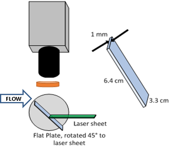
Dr. Todd Lowe, a professor in the Aerospace and Ocean Engineering
Department, is a leader in optical diagnostic tools in fluids and
has extensive experience with PIV in particular. The video below
shows particles flowing over a flat plate (flow direction is bottom
to top). This video is quite remarkable since you can discern
individual particles all the way to the wall. This is a very
challenging measurement that uses fluorescent particles (different
from the ones you will be using in this experiment). As you get
closer to the wall, the laser reflects off the surface of the flat
pate and creates a glare that saturates the camera sensor. As a
result, no particle can be distinguished in the glare region. By
using particles that will absorb the laser light and emit light at a
different wavelength, you can filter out the laser light entirely
(by using narrowband filters on the cameras that will allow only the
scattered light to be imaged). This technique is being pioneered by
Dr. Lowe with support from NASA with some early results below. Note
how well you can see the particles all the way to the wall (the
white line in the video) and how well those particles highlight the
turbulent motion inside the boundary layer.
Figure 1. Fluorescent Particle Image Velocimetry Technique
(courtesy of Prof. Todd Lowe from Virginia Tech) (a)
Experimental Setup, (b) Animation of particle motion as acquired
by PIV camera (flow direction is bottom to top), (c) PIV results
for the velocity magnitude (flow direction is bottom to top ;
dark triangular area in the bottom right corner is the region
shielded from the flow by the flat plate where there is
therefore no significant data).
Partially as a response to the health and safety risks associated
with PIV lasers, researchers at Penn State University proposed an
alternative but similar method to PIV: the Particle Shadow
Velocimetry (PSV). PSV relies on the use of a generalized light
source, such as bright LEDs, which is significantly less expensive
than high-speed powerful lasers. In this configuration, the light
travels along the optical axis of the camera and the measurement
volume (i.e. flow field of interest) is located between the light
source and the camera, see Figure 2. As its name suggests, shadows
of the flow seeding particles are captured in the images obtained
by the camera - you might imagine the result similar to watching a
sunset over the horizon when objects, such as trees, will turn
into silhouettes. Using the proper image processing algorithms,
the images from the camera can be inverted such that they will be
identical to images obtained by PIV systems. Therefore, PSV can
offer the same capabilities as PIV at a significantly reduced cost
while it can also eliminate the high risks associated with using
Class IV lasers. In this experiment, you will be using a
high-speed PSV system to measure the flow field in a
closed-circuit water tunnel in the wake of a cylinder.
Basic principles
While you may be familiar with the operating principles of PIV,
the operating principles of PSV will be introduced in the
following paragraphs. Your experiment will use the same principles
to obtain flow velocity data. The working principle of particle
shadow velocimetry is to capture the shadows of particles in the
flow to allow us to track their position between successively
acquired images. To do so, the flow is imaged by one or two
high speed cameras in order to accurately measure the flow
velocity components. There are generally two types of PSV (or also
PIV) setups: 2-component and 3-component (also known as stereo PSV
or PIV). 2-component PSV uses only one camera and yields 2 of the
velocity components within a plane, whereas stereo PSV uses two
cameras and gives you the full 3 components of velocity over a
thin volume of fluid. Stereo imaging works in much the same way as
how our eyes allow us to accurately perceive distance. Stereo PSV
is more complex to implement and process however, due the addition
of the second camera, so for this lab we will focus solely on a
2-component PSV procedure.
A typical 2-D PSV setup can be seen in Figure 2 below. The light
source is located on the right, where an RGB (red, green, blue)
LED (light emitting diode) light source is used. The light passes
through the flow where flow seeding particles are present. The
particles block the path of the light from the LED as it
propagates to the lens and then to the CCD (charge-coupled device)
sensor of the high-speed camera. In the case of a PSV setup, the
focal plane and focal depth of the lens will determine the region
of the fluid where measurement data is obtained. Only in this thin
volume of fluid will the shadows of the particles will be observed
(i.e. sharp in the image) by the camera. One component of the
optical setup is missing from Figure 2, which is a light diffusing
sheet between the focal plane and the LED light. In the current
experiment, a light diffusing sheet is responsible to evenly
distribute the light arriving from the LED light to the camera.
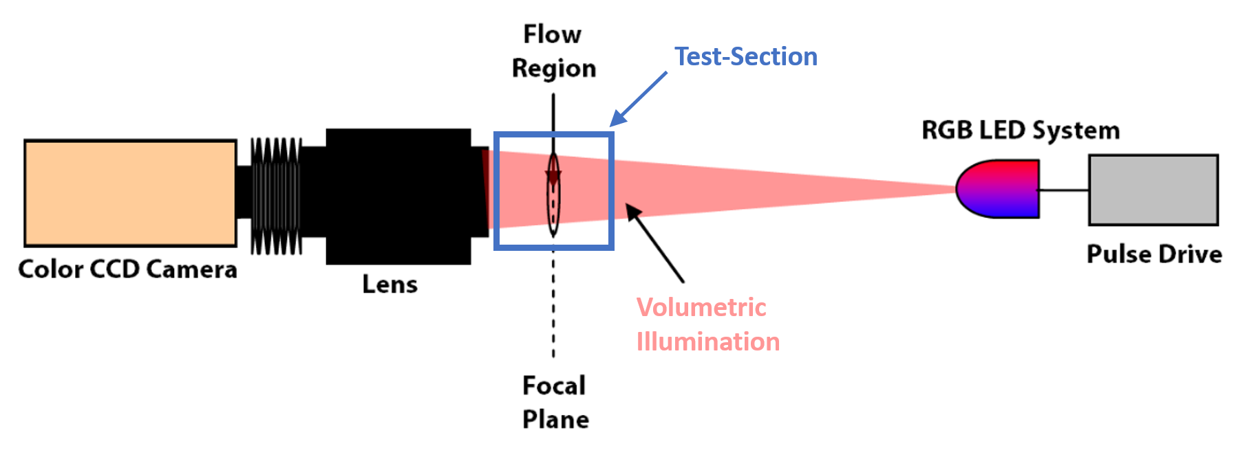
Figure 2. Typical 2-D PSV setup. Picture adapted from INNSI,
found at https://innssi.com/particle-shadow-velocimetry/
Particles
As mentioned above, tiny particles must be present in the flow for
a measurement to be made. These are referred to as seed particles,
or just seeding. It is important that these particles be small
enough to accurately follow all the movements of the flow. That
way, when we measure the velocity of the particles, we are also
measuring the velocity of the flow. These particles are either
dissolved or aerosolized in the flow. Note that, even in well
seeded flows, the particles form only a minuscule fraction of the
volume of the fluid. They therefore have no significant effect
upon the flow. In this experiment, you will be using Cospheric
gray microspheres with a 250-300 micrometer in diameter as seed
particles whose density is identical to that of water, therefore,
they are buoyant in the water tunnel used in this experiment.
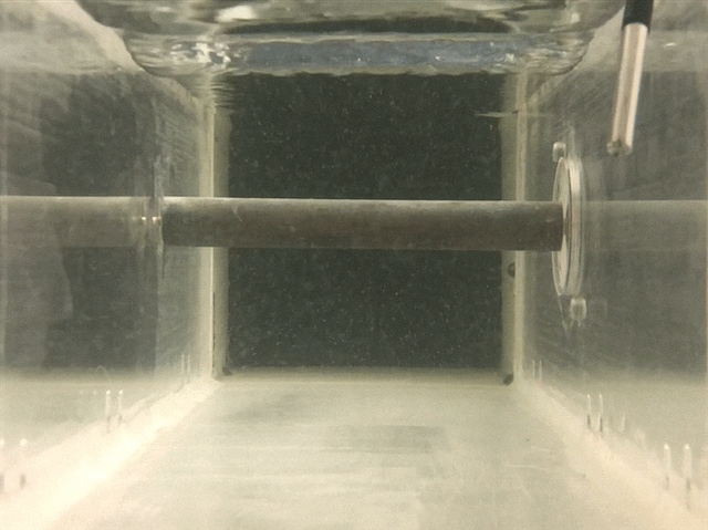
Figure 3. The green seed particles moving in the water tunnel
Light Source
In this PSV experiment, you will be using a time-pulsed RGB LED
light source (seen in Figure 4b), custom designed and built by
INNSI for PSV applications. The light pulses are timed such that
they occur during the time window when the camera is recording the
images. This increases the signal-to-noise ratio of particle
shadows seen in the pictures.
Imaging System
The focal plane of the optical system (camera+lens) will be
located so that it lays in a streamwise plane perpendicular to the
cylinder span, along the centerline of the test-section. The
high-speed camera will be placed perpendicular to the test section
volume as shown in Figure 4b.
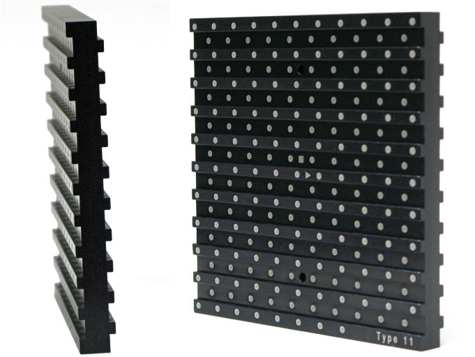
A calibration plate with rows and columns of shaded circles (3.2
mm in diameter and spaced 15 mm apart) is used to precisely focus
the camera and to determine the measurement location. An example
of such plate can be seen in Figure 4a and 4b. The calibration
plate is placed into the test section and the camera lens is
focused to the front surface of the calibration plate. A built-in
software can then accurately determine the relative position of
the camera with respect to the focal plane by acquiring images of
the calibration plate and triangulating the position of each white
circle. An optical calibration is then obtained which is
the relation between spatial units and pixels, i.e. a calibration
constant of pixels/mm is found. From this, the observed particle
displacement measured in pixels is related to particle, or flow,
speed by the software you will be using.
Figure 4. PSV Camera calibration.
(a) Calibration plate from manufacturer LaVision. The dots are precisely located.
Note that some columns of dots are out of plane to allow for
stereo-PSV camera calibration
(to allow for out of plane calibration).
(b) The calibration plate used in the water tunnel.
(c) Side view (looking upstream) of the test volume.
Signals and signal processing
Once the high speed camera is precisely focused, it is
synchronized with the pulses of the LED light so that when you
look at two successive images, the particles will have moved a
couple of pixels. This particle shift between each set of
successive set of images is important for post processing because
the processing code breaks down the images into smaller pieces
called interrogation windows. Within these interrogation windows,
the processing code will compute the cross-correlation between the
interrogation windows of two consecutive images and calculate the
most likely displacement for the entire group of particles inside
the interrogation window. Knowing the time delay between the two
consecutive images, the velocity can be determined. It is
important to note that you want as many seed particles as possible
while still being able to distinguish between the particles for
optimum results.
Once the cross-correlation between a pair of interrogation
windows has been completely calculated, the window shifts over or
down while usually still maintaining a 50% overlap with the
previous interrogation window. This overlap increases processing
time, but it allows for a greatly reduced uncertainty in stitching
all of the interrogation windows back into the full image with
calculated velocity vectors. The processing results in the entire
velocity field in the plane of the laser sheet. With a single
camera, the velocity field measured is two-dimensional (like in
your experiment). For 3D velocity measurements, a second camera is
required and the technique becomes stereo-PSV. From this velocity
field, one can extract information about the flow structures, wake
profiles, and vorticity field. You are encouraged to search for
applications of PIV and PSV measurements in the aerospace and
ocean engineering community before your experiment so that you can
get a wider picture of this method's use and applicability.
2. Apparatus and
Instrumentation
An overview of this experimental setup is provided in the video below:
A. Water Tunnel.
You will be using a water tunnel with a test volume cross section of
6" x 6". This water tunnel, built by Engineering Laboratory and
Design Inc., has a vertical closed circuit arrangement, see Figure
5. On top of the flow circuit is the test section, which is enclosed
by 1/2" thick Plexiglas sheets. The test section has nominal
interior dimensions of 6"x6"x18" and can be operated with or without
a free surface. Flow is driven through the circuit by a 1.5HP
centrifugal pump that can deliver up to 280 gallons per minute. Flow
arrives in the test section through a settling chamber containing a
plastic honeycomb and three 60% porosity screens designed to
straighten the flow, make it more uniform and reduce turbulence
levels. A contraction at the downstream end of the settling chamber
further improves the flow quality by accelerating the flow to test
speed. Flow speed in the test section can be continuously varied
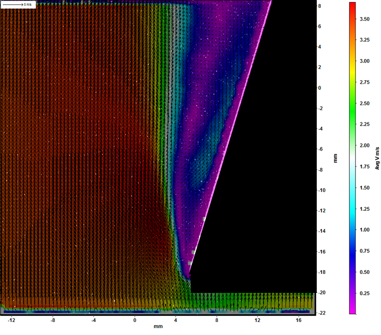
from zero to more than 2.5 ft/s by varying the pump speed. Figure 6 shows the nominal flow speed
and turbulence intensity in the test section as a function of the
pump speed when empty. Note that you can check the set velocity in
the test section yourself using the PSV during your experiment if
you want, and get an idea of the uncertainty by investigating the
properties of the flow outside of the wake.
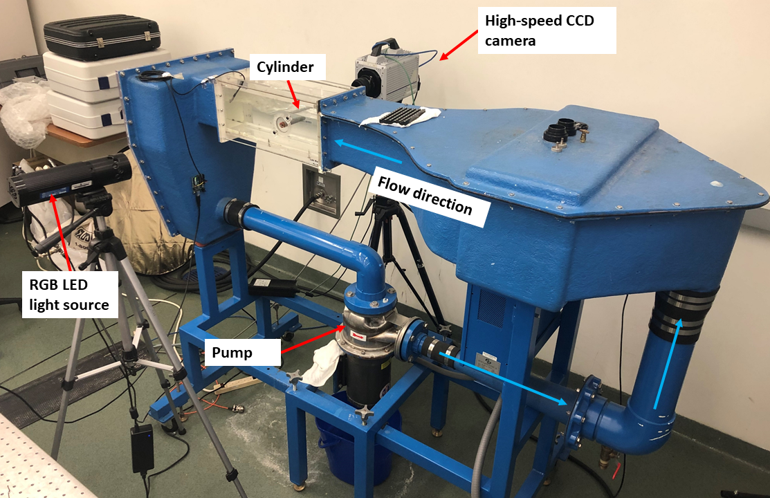 Figure 5. The water tunnel used in this experiment.
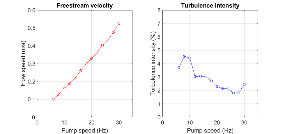
Figure 6. Velocity and turbulence intensity as a function of
pump speed in the empty water-tunnel test section.
The measurements were made 2" downstream of the test section
entrance.
The turbulence intensity is defined as the RMS of the fluctuating
component of the velocity signal (the actual velocity minus its time
averaged value) divided by time average velocity. RMS stands for
'root mean square' which is another term for standard deviation. Figure 7 shows
mean velocity and turbulence intensity profiles measured in the
empty test section for pump speed of 30 Hz.
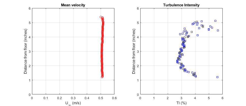
Figure 7. Vertical velocity profiles in the empty test section
2" downstream of the test section entrance for a pump speed of
30Hz. Coordinate y is measured from the bottom of the test
section
The mean velocity is closely uniform varying less than 1% over the
measured distance. Turbulence intensity is about 3% at the center of
the test section. You can get an idea for what this means by
assuming the velocity fluctuations are distributed as a Gaussian, in
which case the velocity would be within two standard deviations
(twice the turbulence intensity) of its mean value 95% of the time.
3% is a fairly high compared to, say, the Stability Wind Tunnel
(0.02%). However, it is not atypical of water flow facilities of
this type.
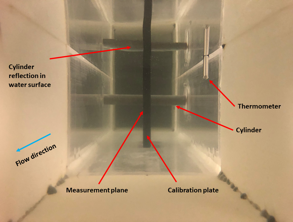
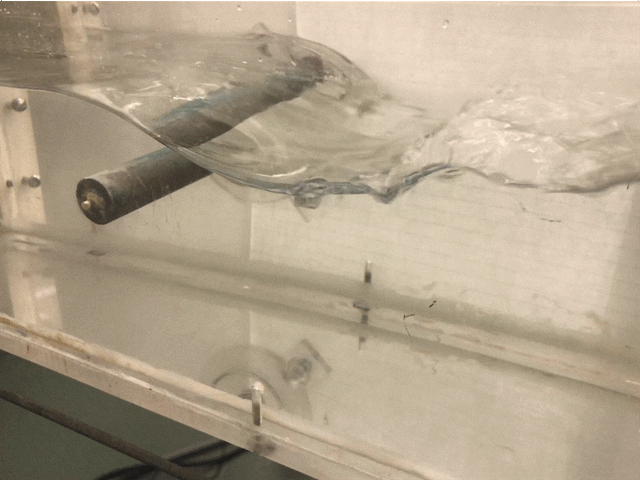
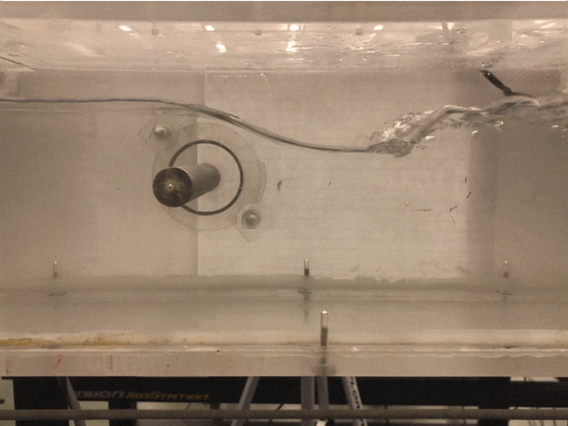
B. Cylinder model
A circular cylinder with 0.75 inches in diameter is mounted close
to the mid height of the test section, see Figure 8. The cylinder
is manufactured from aluminum and spans the entire test section
width (that means, of course, that the ends of the cylinder are in
the boundary layers on the side walls of the water tunnel test
section).
Figure 8. The cylinder in the test section of
the water tunnel.
C. Particle Shadow Velocimetry System
You will employ a 1c2D PSV system (1 camera, 2D velocity
components) for this experiment, see Figure 9. The system uses an
LM2X-DMHP-RGB type 3-Color LED Light Source made by Innovative
Scientific Solutions, Inc. The LED light will be pulsed at 500 ms
intervals for a time period of 180 microseconds.
The camera is a Photron FASTCAM SA1.1 with a 50mm focal length
and an aperture of 8.0. The camera features a 1024 x 1024 pixel
sensor and is capable of 3,600 fps at full frame and up to
500,000fps when using partial frame. In this experiment, the
cameras will image the flow at 200Hz over an area of approximately
10 cm x 10 cm. For this experiment, the 1024 pixels x 1024 pixels
image is broken down into 64 pixels x 64 pixels interrogation
areas.
The fluid motion will be highlighted using gray particles called
microspheres. These particles are manufactured by Cospheric to
have a diameter between 250 and 300 microns and a density of 1
gram/ccm.
The system will be calibrated prior to your laboratory session.
However, the PSV system does not require the recalibration (unlike
PIV) as long as the camera and lens settings (focal distance and
aperture) is not modified. Taking a benefit of this feature, the
camera and the light source has been mounted on a table with a
traversing system responsible for moving the light source and the
camera in the streamwise direction. You will therefore have the
freedom to choose where to take data with the PSV system within
the entire volume of the test section.
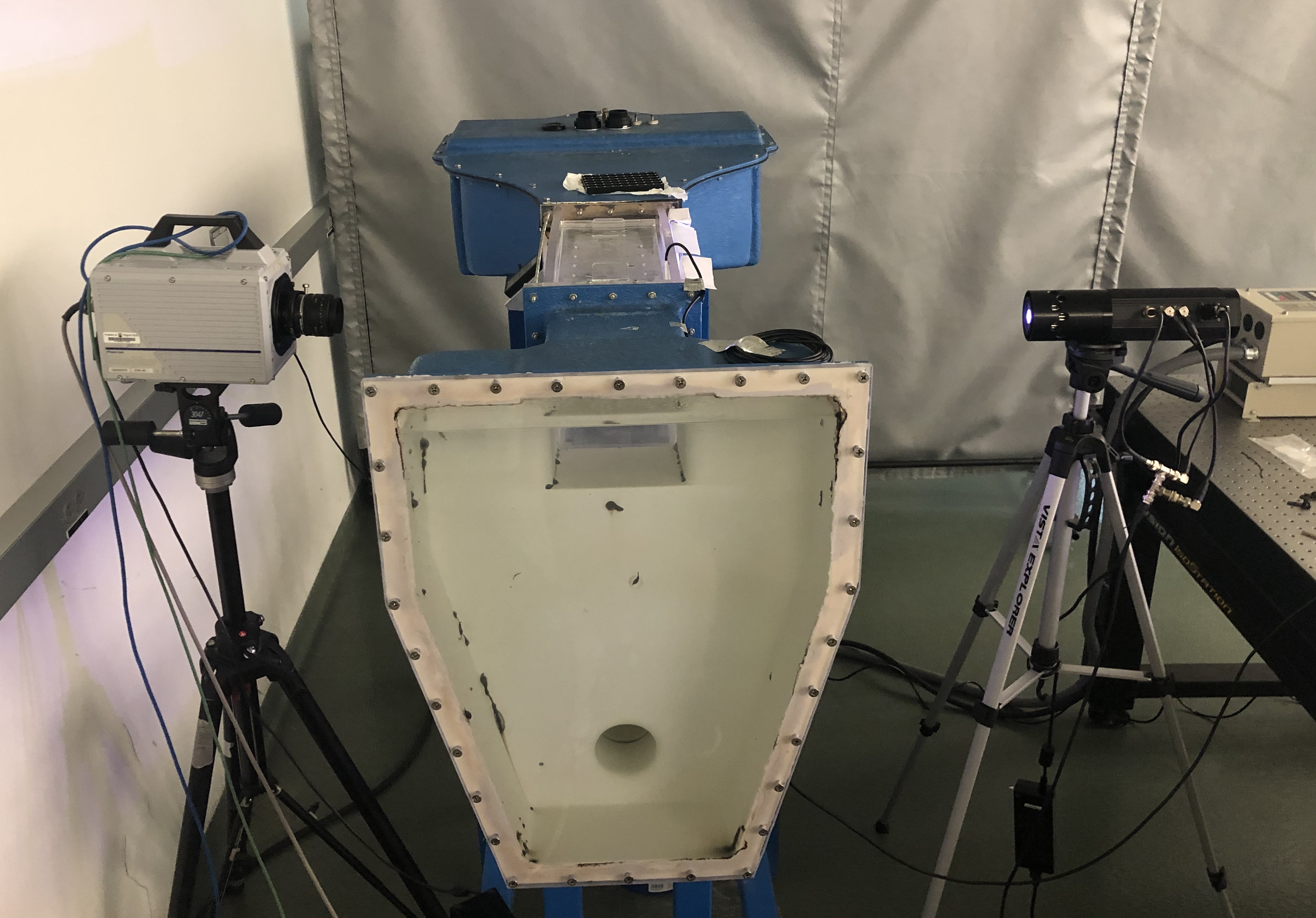
Figure 9. The overall view of the PSV setup in
the water tunnel.
D. Traversing system
The high speed camera and the light source are mounted on an
aluminum bar and can be traversed along the streamwise direction
using a VelmeX traversing stage and a linear bearing. The former is
responsible for positioning the optical system while the latter
carries the mechanical load. You can use the traverse to vary the
location of the field of view in the streamwise direction. This
allows you to acquire data both upstream and downstream of the
cylinder.
The CAD view of the traversing system is shown in Figure 10, while a
close-up annotated picture of the system is shown in Figure 11. Note
that the "home" of the traverse is at the downstream end of the
traversing axis, corresponding to X=0 in with X increasing upstream
of this location. The traverse can be operated using the Matlab GUI
shown in Figure 12. You can run the GUI from "D:\AOE3054_MatlabGUIs"
and typing SingleAxisMotion in the Matlab command window then
hitting enter. First, connect to the traverse using the "Connect
Traverse" button. You can use the "Refresh Traverse" button to
update the Current X position of the traverse carriage. Use the New
X Abs input box to set a new requested X location (absolute
coordinate) and click on the Move X button to move the traverse. Please
make sure to return the traverse carriage to X=0 in at the end of
your session to help the next group.
You will be using two coordinate systems: one is the coordinate
system of the traverse (1D with +X being opposite to the flow
direction) and the coordinate system of the PSV (2D: x,y). You will
need to keep log of where the traverse system is set and a
coordinate transformation will be provided to you that links the PSV
coordinate system and the traverse coordinate system.
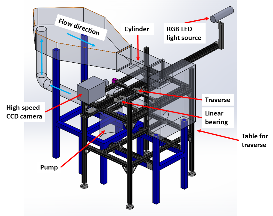 Figure 10. The CAD view of the traversing system and
the PSV apparatus.
Figure 10. The CAD view of the traversing system and
the PSV apparatus.
The water tunnel has been made transparent to improve
visibility.
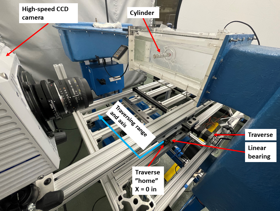 Figure 11. The close-up view of the traversing
system.
Figure 11. The close-up view of the traversing
system.
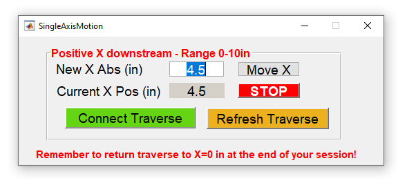
Figure 12. The Matlab GUI used for
controlling the traversing system.
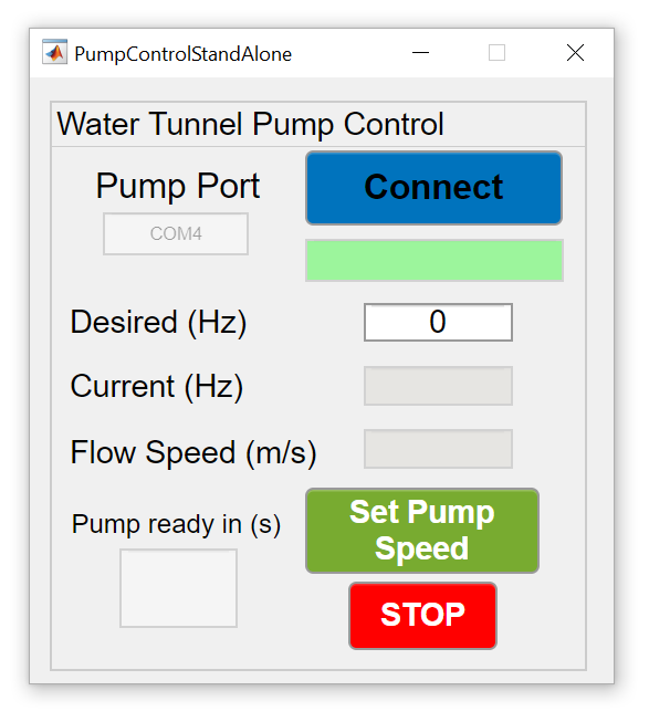
E. Operational instructions
During your experiment, you will be changing the pump speed
using the Matlab GUI interface shown in Figure 13(a). You can run
the GUI from Matlab after navigating to the following directory:
"D:\AOE3054_MatlabGUIs". The GUI can be run by right clicking on
file "FanControlStandAlone_App.mlapp" and choosing the "Run"
option as shown in Figure 13(b). The software will ensure that the
inverter driving the motor of the pump will follow the speed (in
unit of Hz) you set in the GUI. The software contains all safety
features necessary for you to operate the pump over a wide range
of conditions in a continuous manner. The lowest speed the pump
can operate is 6 Hz, and the highest speed is 30 Hz. Below 6 Hz,
the AC motor driving the fan would not obtain sufficient amount of
cooling, and above 30 Hz, the flow starts interacting with the
ceiling of the water tunnel. You can operate the tunnel using the
following steps:
-
Connect to the pump controller using the Connect button. Once
successful, you will be prompted the "Connected" message in the
status indicator.
-
Set a desired speed in Hz (anywhere between 6 Hz and 30 Hz)
and click "Set Pump Speed". The pump speed will stabilize in 10
seconds, the GUI will countdown from 10 to 0 s and will prompt you
the Current speed in Hz and the current flow speed in m/s.
-
You can stop the pump by clicking the STOP button. Make
sure you stop the pump once you finished acquiring data and/or
at the end of your lab session.
You will have access to the water tunnel using PTZ (pan tilt
zoom) cameras. You are encouraged to take screenshots of the
apparatus as they are operated for your logbook and to move the
PTZ camera around to get a better view of the equipment and the
measurement apparatus.
F. Instrumentation for Measuring the Properties of Water
Unlike air, the properties of water are remarkably constant with
pressure (an increase in the atmospheric pressure by a factor of
100 would only have a 0.5% effect on density). They are however a
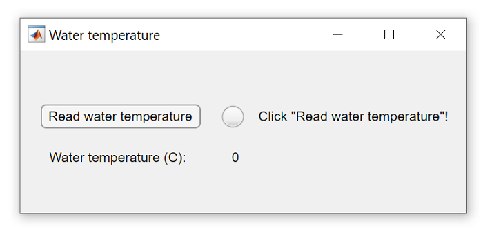
function of temperature. You will use another Matlab GUI that
obtains readings of the water temperature using a waterproof
DS18B20 digital temperature sensor (see Figure 4) operated by an
Arduino Uno board. According to the manufacturer, the sensor has a
±0.5℃ accuracy within the -55 and 125℃ temperature range. In
Matlab, you can run the GUI by right clicking on its name
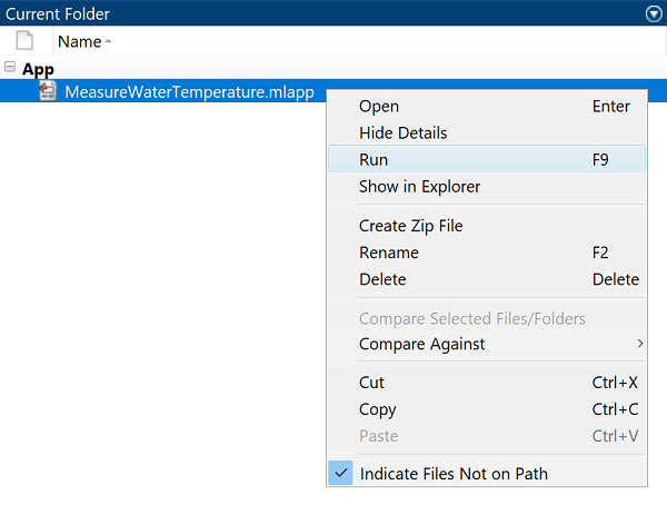
("D:\AOE3054_MatlabGUIs\MeasureWaterTemperature.mlapp") and click
on Run. Once ready, click on the "Read water temperature" button,
which will obtain a temperature reading, see Figure 15. The
measurement takes less than a minute. Repeat the measurement as
many times you need throughout your experiment.
Figure 15. Obtain water temperature using the
Matlab GUI.
Tables for the density and kinematic viscosity of
water can be found in numerous textbooks (e.g. Shames, 1992). The
following calculator uses a quintic fit to these tables. The
uncertainties in the curve fits are ±4x10⁻⁹ m2s-1
and ±0.04kg m-3
G. Coordinate system
You will be using two coordinate systems during your lab session,
one is the coordinate system of the PSV equipment and the other is
the traverse system, see Figure 16. The PSV coordinate system is
defined at the downstream end of the cylinder while the traverse
coordinate system points in the opposite direction and it is
measured from the "home" of the traverse. In your lab report, you
will be expected to use a third, global coordinate system. On the
desktop of the computer running the experiment, you will find a text
file called "CoordinateTransformation.txt" which will contain the
current information on how to relate the two local coordinate
systems to each other.
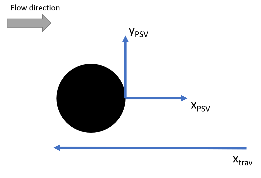 Figure 16. The coordinate systems used in the experiment.
3. Theory
A. Ideal flow model of flow past a circular cylinder
In AOE 3014 you studied irrotational incompressible flow past a
circular cylinder without circulation (see Bertin, 2001, Section
3.13). Such a flow can be generated by adding a uniform flow, in the
positive x direction to a doublet at the origin directed in
the negative x direction. Of particular interest here is the
velocity distribution predicted by the theory which is given, in
terms of polar coordinates and components centered on the cylinder
axis, by the relations:
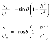 .........................(1)
where the symbols are defined in Figure 17 and R is
the cylinder radius (D/2). In terms of Cartesian
components and coordinates centered on the cylinder axis, the same
velocity field is:
.........................(1)
where the symbols are defined in Figure 17 and R is
the cylinder radius (D/2). In terms of Cartesian
components and coordinates centered on the cylinder axis, the same
velocity field is:
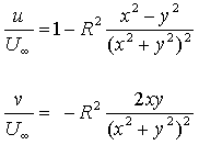 .........................(2)
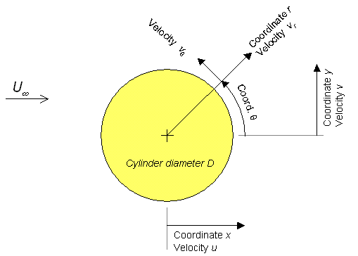
Figure 17. Definition of coordinates and components for
cylinder flow theory.
4. Practical Work
A. Getting familiar with the equipment and ready for an
experiment
The following procedures are designed to help you get a feel for
the water tunnel, the cylinder model and the PSV software. Feel
free to play with the apparatus at this stage, but don't forget to
record any results, thoughts, ideas or concerns in the logbook.
Setting up a PSV experiment to make a measurement from scratch can
take days, so don't feel frustrated if, in the space of a 2-hour
45-minute lab, the measurements don't go too quickly or the data
rate is slow. You are obtaining research-quality measurements
using cutting edge technology, each data set you get is a
significant achievement.
For information regarding software instructions, see section 7.
- The PSV system will have already been turned on by your lab TA
and will be ready for use when you arrive in the lab.
- Acquire a data set and look at the raw images. Do you see the
cylinder? Do you see the particles? Are they moving with the
flow?
- Note that you need to ensure that the overhead lights (directly above the water tunnel) are turned off (ask your TA for assistance). Since you are acquiring images at 200Hz,
the 60Hz flickering of the lights will lead to variations in the brightness of the particles seen by the camera and contaminate your measurements. An illustration of this is provided in Figure 18 below:
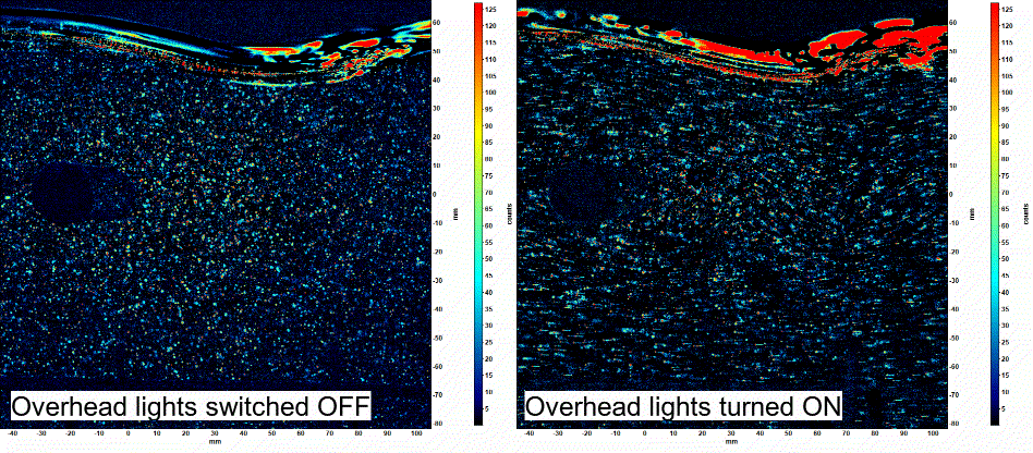 Figure 18. Impact of overhead lights on particle brightness (animation extracted from Bright field correction results from the DaVis software).
- Export the mean velocity field and look at the magnitude of
the vectors? What is the freestream velocity? What is the
velocity in the wake? Do these make sense? Are they consistent
with Figure 6? Discuss among the group what it shows. Also,
discuss in the group where in the flow you expect the vertical
component to be large.
- Try changing the flow speed using the Matlab GUI. How does
speed affect the PSV measurement? Does it work just as well?
Think about a good flow speed to measure at.
- Note the water temperature again. Has it changed? Will you be
able to assume its constant, or will you have to re-measure it
periodically? Can you estimate the cylinder Reynolds number,
from the velocity measurement outside of the wake and the
temperature? What flow regime shall your measurements fall based
on the Reynolds number?
B. Designing and Implementing an Experiment
When you feel comfortable with the equipment it is time to choose
some goals and decide on a strategy to achieve them. Suggested goals
are given below. Of course, you are encouraged to choose a different
goal of your own, or adapt these goals, but the goals you end up
with must be scientific, and clearly stated in the logbook. Note
that, as always, your grade does not depend upon how many goals you
achieve, but on how complete, careful, scientific and documented
your work is. Neither does your grade depend upon how close your
results agree with any other pre-conceived ideas of what the answers
should be. Instead it depends upon how open mindedly and objectively
you assess your results, their qualities and limitations, and what
they appear to show. Also, remember that processing the PSV data
will be time consuming (about 5-6 min per data set), so structure
your measurements such that you can achieve your goal(s) even if you
end up getting fewer measurements than may initially seem possible.
When planning your objectives and measurement schedule, count on the
PSV to acquire data in about 1 min.
Goal 1. Design and implement a series of tests to
determine the shape and form of the circular cylinder wake at the
center span at a fixed Reynolds number.
Suggestions. Don't forget to record and explain your
choice of conditions (i.e. flow speed) and measurement locations
in the logbook. If you measured wake structure in Experiment 3, at
the much higher Reynolds number of the wind tunnel, measuring at
some of the same streamwise locations (relative to the cylinder
center and its diameter) would also provide a valuable comparison.
Its usually easiest to measure the wake in a series of vertical
profiles. Don't forget you can measure both vertical and
horizontal velocity components. (If you measure both vertical and
horizontal mean velocities at the same actual points you can
determine the magnitude and direction of the mean velocity vector
at each point). Analyze and plot your results as you go.
Re-measure any funny looking points. Keep careful documentation of
what you do, why you do it, set up characteristics, expected
results, unexpected results, analysis, photos and plots in the
electronic lab book as you proceed. Ideally, you would want to
measure the velocity upstream of the cylinder (since it is the
freestream velocity you will use to normalize all your results).
You can traverse the light and camera to image the flow upstream of the cylinder to do so.
Make you are carefully documenting where you take this measurement. Will this measurement be
contaminated by the presence of the cylinder? How so? Could you
use the continuity equation to work out the free-stream velocity?
How does that compare to the data the Matlab GUI prompts you?
Analysis suggestions for later. Basically, you want to
present and describe your mean velocity flow field as clearly as
possible, reveal the shape and form of the flow, and compare that
with Experiment 3 or any theoretical model you are aware of. When
post-processing your data, try using the mean velocity field
information to visualize the streamlines of the flow. Mean
velocity profiles show the time average shape of the flow. Look at
the individual images. They show what the flow looks like at each
instant. Linking these views is good discussion.
Goal 2. Design and implement a series of tests to
examine the flow over the front of the cylinder at center-span a
set Reynolds number, and compare with ideal flow theory.
Suggestions. The issue here can be "how good is the ideal
flow solution over the front of the cylinder, since the flow here
isn't separated". Record and explain your choice of conditions for
your measurement (i.e. flow speed) and measurement locations in
the logbook. Choose your measurement locations to make the
comparison with the theory as straightforward as possible. Don't
forget you can measure both horizontal and vertical velocity
components. Determine how you can obtain vorticity from the
velocity field. Checking the freestream velocity outside the wake
of the cylinder might be a wise thing to do since knowing the free
stream velocity is critical to compare with the theory. Analyze
and plot your results as you go. Re-measure any funny looking
points. Keep careful documentation of what you do, why you do it,
set up characteristics, expected results, unexpected results,
analysis, photos and plots in the electronic lab book as you
proceed. Analysis should include uncertainty estimates for all
results.
Goal 3. Identify the flow regimes the cylinder generates
in its wake by mapping out the flow's Reynolds number, Strouhal
number and induced drag.
Suggestions. Calculate the Strouhal number using
instantaneous velocity data, calculate the drag coefficient using
time-averaged velocity data. Plot the results as a function of
Reynolds number and compare it to other measurement results (see
Ref 3). How does your results differ and why? How does the
turbulence intensities differ from the data presented in the
literature? How does the Strouhal number change with flow speed?
How does this compare to data presented in the literature?
Time management
The group should leave few minutes at the end of the lab period
for discussion and to check that everybody has everything they
need.
You will need to use your own cloud server (such as Google Drive
or Dropbox, etc.) to transport your data from the lab
computer running the experiment to your own device. Make sure
you have access to a cloud service. Within your cloud, you will
need 350 Mb of free space per one instantaneous data set. For
time-averaged data, you will need 10 Mb of free space. Prior
to your experiment, make sure you prepare enough space in
your cloud and include the link to your cloud provider in your
logbook. Use a web browser on the laboratory computer
during your lab session to upload your data to your cloud.
Alternatively, you may use a file sharing website, such as this one, to transfer your
data from the PSV computer to you own. Keep in mind that data
transfer might take up to 15 minutes.
5. Recommended Report
Format
Before starting your report read carefully all the requirements in Appendix 1.
Title page
As detailed in Appendix
1 .
Introduction
Begin this section by stating logical objectives that fit what
your data has shown you.
Then explain in summary form what was done to achieve the
objectives. You could follow this with a background discussion of
what PSV is and what sources of error there are and/or a
description of the basis of ideal flow theory for the circular
cylinder. If you can draw on any material additional to the manual
that is good. Finishing with a summary of the layout of the rest
of the report would work well.
Apparatus and Instrumentation
This section is probably easiest to write in two parts (though
that is not required), one dealing with the water tunnel and the
other with the PSV. In describing the water tunnel give all
details relevant to the experiment (e.g. closed circuit,
contraction ratio, dimensions and shape of test section, flow
quality in the empty section at test conditions, flow speed range
and control etc.) You might include here some of your measurements
(e.g. of the inflow velocity) if they are relevant to describing
the characteristics of the facility, as opposed to the cylinder
flow. Also describe the model, its dimensions, its method of
mounting, its vertical position when mounted, the traverse its
accuracy etc. In describing the PSV, explain what type of system
was used, its optical characteristics, the components of the
system, the location of the measurement volume in the test
section, software etc..
To describe all of this, diagrams and/or labeled photographs,
screenshots are very necessary. Take what you like from the
manual, but be sure to reference it. You will have to show at
least one figure showing the water tunnel test section, model, and
model mount in relation to the PSV measurement area. Make sure
your figure(s) are dimensioned properly. Include your
uncertainties in primary measurements in this section
Results and Discussion
A good way to begin is to briefly state what measurements were
made and at what locations and conditions. You should also include
here definitions of the statistical quantities plotted (e.g. mean
velocity, mean vorticity etc...), and explanations of how their
uncertainties were calculated and what those uncertainties were.
You should reference a table (copied out of your Excel file) or
appendix containing the uncertainty calculation. Early on in the
results and discussion (or even in the apparatus and
Instrumentation) you need to define a coordinate system, and any
key normalizing variables, using a diagram and description in the
text, e.g. "The coordinate system to be used in presenting results
is shown in figure ??. Coordinate x is measured downstream
from the cylinder center, y vertically upwards from that
center and z, directed so as to complete a right-handed
system is measured from the center span location. Velocity
components u and v are defined in the directions x
and y. Distances will in general be normalized on the ???
and velocities on the approach velocity measured at x=??,
y=??, z=?? )".
If you have them, now would be a good time to introduce any
flowvis pictures. Don't just describe what the static pictures
show, use the pictures as a springboard to describing what you
actually saw.
Next introduce your profile plots - the kind of wording
suggested in experiment 3 will work just fine here. Now describe
in detail the plots and error estimates. Then discuss what their
significance is given the goals/ objectives you have chosen (look
again at the suggestions given with the goals above). One workable
approach is to describe what appears on each of the plots in turn,
using a separate paragraph for each, inserting sentences of
discussion as you go e.g. "Figure ?? shows the profile of uRMS
(normalized on free-stream velocity) plotted against y
measured at x=?? and z=??. At the limits
of the profile, turbulence levels are low at about ?? and
reasonably consistent with values measured in the empty test
section of ?? (see AOE 3054 Course Manual, 2016, Experiment 4).
Presumably these points lie outside the cylinder wake. The wake
edges appear to be marked by the large increases in uRMS
at around y=?? and ??. The fact that velocity
fluctuations in the wake should be larger than outside is
consistent with turbulence being present in...".
Make sure your results and discussion include (and justify) the
conclusions you want to make and that those conclusions connect
with your objectives (if not, change the discussion or the
objectives).
Conclusions
Begin this section with one or two sentences describing what you
did. Then draw your conclusions, each numbered and starting on a
separate line. Each conclusion should summarize an important piece
of information that was revealed or taught by the experiment. Make
sure the conclusions cover all the points addressed by your
objectives and all the important points of your discussion. Note
that no new material should appear in the conclusions. It should
be possible to write them by simply lifting key sentences from the
rest of your report (mostly the Results and Discussion). Also note
that the conclusions should stand by themselves, though you may
refer to the figures if you wish.
6. References
- Bertin J.J. 2001, Aerodynamics for Engineers , 4th
edition, Prentice Hall.
- Shames I. H., 1992, Mechanics of Fluids, Third
Edition, McGraw Hill, New York.
- Panton R. L., 2013, Incompressible Flow, 4th edition, Wiley,
New York.
7. Addendum: Running the
PSV Software
Compile your logbook on a different computer to that running the PSV
software.
Follow the software step-by-step instructions below. It is paramount
that you follow these directions precisely as the data acquisition
software is complicated and error that you make while using it can
compromise its delicate setup.
If the PDF below does not display properly, you can download it manually here.
You should now be ready to use this system to meet your goals. Don't
forget when taking the next or any subsequent measurement to change
the name of the output file or the old data will be overwritten.
Each run will generate a series of 200 images and DaVis will export an associated set of 199
data files for the instantaneous velocity field and 9 files for the average quantities (Keep in mind that exporting data does take several minutes).
You can use a combination of exported data and screenshots from the DaVis results for your logbook,
but keep in mind you will need all your data files exported for the analysis in your report.
Store your data (instantaneous and averaged) for each run in separate folders. You can then download this
PIV Data Matlab Importing package - Updated 14 Sep 2021
to import the data from all your files (the 199 instantaneous and 9 averaged quantities) within a set and consolidate it in matrix form in Matlab.
You can then use these MAT files and write your own codes to perform further analysis and generate plots. A description of the contents of this package is provided below:
Content of the AOE3054_PIV_Import_Rev1 Package:
- AOE3054_PIV_ImportInstant_2020.m: you will run this function on the 199 instantaneous velocity files
to import that data into Matlab. The code will create a MAT file (whose name you will specify) with four variables:
- X and Y are the streamwise and vertical coordinates of the measurement locations. The X and Y matrices have a size of MxM.
- U and V are the velocity component matrices and will be MxMx199 matrices since you obtain components for each consecutive pair of the 200 images.
- AOE3054_PIV_ImportMean_2020.m: you will run this function on the 9 averaged
quantity files to import that data into Matlab. The code will create a MAT file (whose name you will specify) with 12 variables:
- X and Y are the streamwise and vertical coordinates of the measurement locations
- U and V are the velocity components at those points
- Umag is the velocity magnitude
- stdU and stdV are the standard deviation at each point on the grid (computed over the 200 images)
- AKE and TKE are the average and total kinetic energy
- Rxx, Rxy, and Ryy are the Reynolds stresses
- Two folders containing a sample data set are provided in the ZIP file so you can test the import codes and debug your own plotting codes ahead of your experiment:
- 20HzSampleData_Instantaneous: 199 instantaneous velocity files acquired at a pump speed of 20Hz.
- 20HzSampleData_Averages: 9 averaged quantities acquired at a pump speed of 20Hz.