Most measurement systems may be broken down into 3 components; (i) a detector or transducer that senses the physical quantity of interest and transforms it into a mechanical or electrical signal, (ii) an intermediate stage that amplifies or otherwise modifies the signal, and (iii) a final stage in which the signal is displayed or stored.

A simple example of such a measurement system is the mercury thermometer. The mercury in the bulb senses a change in temperature through thermal expansion or contraction. This mechanical signal is amplified by the capillary tube attached to the bulb - a small change in the volume of the mercury producing a large change in its height in the capillary. Finally the temperature is displayed by comparing the height of mercury with a scale on the outside of the tube.

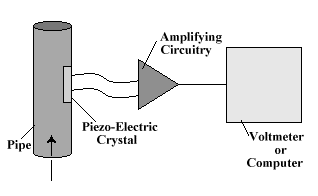
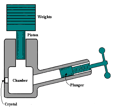
A slightly more complex example, perhaps better representative of those measurements systems often seen in aerospace or ocean-related experiments, is the pressure gage shown in figure 1. This particular gage uses a detector known as a piezoelectric crystal to detect the fluid pressure at a pipe wall. When compressed such a crystal produces a small voltage across its faces. An electrical circuit is then used to amplify this voltage. The resulting signal is then displayed using a voltmeter or perhaps read into a computer and stored.

It is obvious that to use a measurement system you have to know the relationship between its output and the quantity it senses, called a calibration. You also have to know the limitations of the system, specifically its range, its accuracy, precision and repeatability, and how quickly it can respond to a change in the quantity being measured, called its dynamic response.

1.1 Calibration
To calibrate a measurement system you have to compare its output with a known input. Consider, for example, the pressure gage of figure 1. This device could be calibrated by mounting the transducer in a closed vessel with a piston at one end, as shown in figure 2. (Such a vessel is called a dead-weight tester.) Placing a weight on the piston produces a known pressure in the vessel equal to the weight divided by the piston area. 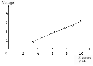After applying a series of weights and measuring the corresponding output voltages of the pressure gage we can plot the relationship between the output voltage and pressure (figure 3). Mounting the transducer back in the pipe we now use this calibration curve to convert voltage readings into pressures at the pipe wall.

As a general rule it is unwise, if you have the choice, to trust a calibration made by a manufacturer or estimated through a theoretical calculation - measurement systems rarely work exactly as they are supposed to. Repeating a calibration at regular intervals is also a good idea since it may drift with time or ambient conditions. Having a repeatable and accurate calibration is obviously a prerequisite for an accurate measurement.

1.2 Range
The design of a measurement system obviously limits its range - the thermometer cannot measure temperatures for which the mercury contracts into the bulb or blows off the top of the capillary, the pressure gage cannot measure pressures for which the voltage is greater than that which can be handled by the electrical amplifier. While staying within the design limits is often important if the measurement system is not to be damaged, staying within the calibration limits is important if accurate measurements are required. For example, the calibration curve of figure 3 only extends from 3 to 10 psi. Using the pressure gage to measure a pressure of 1 psi almost certainly would not break it, but one would need to extrapolate the calibration curve downwards. There is no guarantee that such an extrapolation would be accurate.

1.3 Accuracy and Precision and Repeatability
Accuracy is merely an optimistic word for error, the difference between the output of a measurement system and the true value. (When we say that a probe measures velocity to an accuracy of 1 ft/s we mean that its measurements are in error by that amount.) Much of the error in a measurement system can be eliminated by calibration. However, drift, lack of repeatability and inaccuracy in the calibration mean that there will always be some residual error.

Precision is the resolution with which a measurement may be made. For example if the thermometer has graduations every 2 degrees it probably could be read with a precision of about half that. Precision does not guarantee accuracy. The thermometer scale may have been printed in the wrong place making it 10 degrees in error.

Repeatability is the difference between successive measurements of the same quantity.

1.4 Static and Dynamic Response
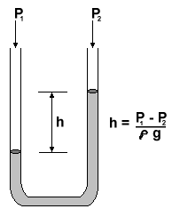
Static response refers to the behavior of a measurement system when it is used to measure a fixed quantity. Dynamic response refers to behavior when the quantity is changing with time. The U-tube manometer (figure 4) is a measurement system that gives a good physical feel for the difference between static and dynamic response. Such a manometer senses the pressure difference between its two open ends through the displacement of a column of fluid in a vertical U-shaped tube.

For steady pressure differences (p) the displacement of the manometer fluid (h) is given by hydrostatics,

     (1)

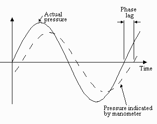
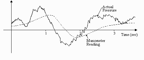
For pressures that are changing with time, equation (1) only holds if the changes are of very low frequency - a fraction of a Hertz. This is because, as the frequency is increased, inertia of the fluid column and friction between it and the tube start becoming important. Thus, the motion of the fluid column begins to lag behind the pressure change and the amplitude of this motion begins to differ from that given by equation 1 (figure 5).

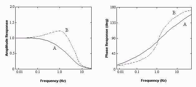
We refer to the ratio of the amplitude of the pressure fluctuations indicated by the manometer to the actual amplitude as the "amplitude response". We refer to the lag of the manometer, measured in terms of the angle of the sinusoidal fluctuation as the "phase response". If we apply a series of sinusoidal pressure fluctuations of different frequencies we can plot the amplitude and phase response as functions of frequency (figure 6). These curves define the "dynamic response" of the manometer.

Most U-tube manometers tend to have dynamic response curves that look like A or B of figure 6. Curve A is for a small diameter tube in which viscous friction between the fluid and tube wall is sufficient to damp out much of the oscillatory motion of the manometer fluid that fluctuations in the pressure being measured are trying to induce. Curve B is for a manometer with a broad tube that will damp these oscillations to a much smaller degree. At some frequencies the amplitude response is actually greater than 1 (indicated pressure fluctuation greater than actual). These are frequencies close to that at which the manometer fluid would naturally oscillate back and forth in the U tube. Both curves show that the amplitude response of a manometer becomes very small (and for the most part useless) when subjected to pressure fluctuations at frequencies greater than a few Hertz.

The fact that we have used sinusoidal pressure fluctuations to define the dynamic response of our manometer may seem somewhat artificial. In reality, however, it helps us predict how the manometer will respond to any signal. Consider, for example, the pressure signal shown in figure 7 (produced perhaps by an unsteady fluid flow). Such a signal contains many frequencies. If the manometer operates as a linear device its response is the (linear) sum of its phase and amplitude response to each of the frequencies in the signal. i.e. it will respond mostly to the low frequency parts of the signal.

A manometer is obviously a measurement system with a poor dynamic response. Many (usually electrically-based) measurement systems can respond much faster to changes in the quantity they measure (at frequencies of kHz or even MHz). However, they are all ultimately limited in much the same way.

2.1 Mean, standard deviation and histograms
Once a series of measurements has been made the engineer is faced with the task of interpreting them, i.e. deciding what they mean. This is often a lot more difficult than it sounds. Imagine, for example, a test to examine the behavior of a wing spar. An engineer places a position sensor on the spar and records the signal from it at cruising conditions. What do the measurements (the recorded signal) mean? Do the say anything about the average load on the spar? Is the spar vibrating excessively? Could it be in danger of developing a fracture? Answering these questions does not only require a physical and theoretical understanding of the situation but also requires some analysis of the measurements made.

In this, and many other, situations a good first step would be to calculate the mean and standard deviation of the measurements. The definitions of these quantities depend on whether the data from which they are to be calculated are discrete (i.e., a sequence of measured points) or continuous (e.g., an electrical signal). For a set of N discrete samples of a quantity x the mean  and the standard deviation _x are given by the relations

     (2)

     (3)

In our example the mean of each signal would be the average deflection of the spar which presumably could be used to estimate its average load. The standard deviation or variance are measures of how widely the measurements are spread around the mean (i.e., how large, on average, (x_i - )² or (x(t) - )² are). In this case (assuming the position sensor had a good dynamic response) they could be taken as indications of the intensity of vibrations in the spar. For obvious reasons, the standard deviation is often referred to as the "root mean square" or r.m.s., especially when dealing with electrical signals. Since such signals are often sinusoidal it is useful to remember that the r.m.s. of a sinusoid is 0.7071 of its amplitude, verify this for yourself using equation 3.

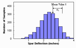
There are many other ways of presenting data in a statistical way. Perhaps the most revealing is a histogram. To construct a histogram the range of the quantity being measured (deflection in our example) is divided up into a number of equal intervals, or 'bins'. For discrete data we then merely add up the number of samples falling in each bin. For continuous signals we add up the time for which the signal lies in each bin. The result is a graph showing how the data are distributed. In our example, such a histogram could show whether our spar had ever deflected sufficiently to yield. The mean and standard deviation may be represented on a histogram, as shown in figure 8. The mean, being a measure of the average, lies near the center of the histogram. The standard deviation, being a measure of the spread, is usually about one quarter to one sixth of the width of the histogram.

2.2 Probability density functions - the normal distribution
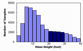
There is a close connection between histograms and probability. Consider, for example, measurements of the heights of waves hitting an oil rig during a season. A histogram of these measurements (see figure 9) can be used to estimate the probability of waves of a certain size hitting the oil rig in the future. For example, the probability of a wave with a height (H) between 20 and 30 feet hitting the rig may be estimated by adding up the number of samples in bins in the range 20 < H < 30 and then dividing by the total number of samples in the histogram. This is equivalent to taking the ratio of the area of the histogram between H = 20 and H = 30 and dividing by the total area, see figure 9.

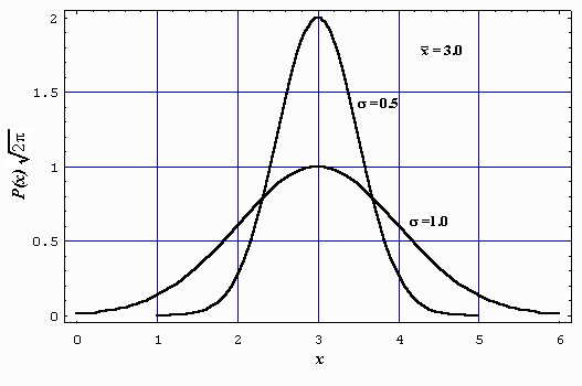
The natural extension of this is the probability density function, which is defined in terms of its area as follows.

"Consider a probability density function p(x) of a quantity x (in the present example, wave height). The area under p(x) between two values x₀ and x₁ is the probability P that a given sample of x will fall between x₀ and x₁."

Mathematically this may be written as

     (4)

     (5)

     (6)

     (7)

     (8)

     (9)

     (10)

     (11)

Example
A sensor is used to detect the flow rate of fuel to a jet engine. Due to electrical interference in the instrumentation used, however, successive readings from the sensor fluctuate. The following are 21 such readings (in arbitrary units),
 

Reading   Flow rate   Reading   Flow rate   Reading   Flow rate
1         .512        8         .734        15        .627
2         .477        9         .771        16        .701
3         .794        10        .486        17        .573
4         .672        11        .559        18        .721
5         .713        12        .614        19        .802
6         .588        13        .687        20        .553
7         .621        14        .722        21        .605

From equation 2 we have 

and, 

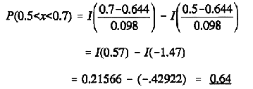
(b) Assuming the readings are distributed normally calculate the probability that a reading taken at random will have a value between .5 and .6.

 Applying equation 10 we have,

(c) What percentage of a large number of readings are likely to lie above a value of .8?

 Applying equation 10 again,

i.e. 5.6%

(d) What percentage of a large number of readings are likely to lie within two standard deviations from the mean?

We have

i.e. 95%. Alternatively we could say that there is a 95% probability that a reading will lie within two standard deviations of the mean.

2.3 Linear regression
Linear regression is the process of fitting the best possible straight line through a series of points. Linear regression is often used to reduce a set of calibration points to a simple mathematical relationship (that can, for example, be implemented on a computer) or deduce the underlying trends from a set of measurements that are expected, on theoretical grounds, to follow a straight line.

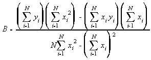
Consider a series of measured points (x_i, y_i) describing a relationship between two quantities x and y. (A good example here is the measurements of voltage and pressure we would have got in our calibration in section 1.2). We wish to find a straight line of the form

     (12)

     (13)

     (14)

     (15)

     (16)

     (17)

(18)

     (19)

     (20)

     (21)

Almost all engineers in the "real world" deal in one way or another with data derived from experiments or tests. They may have obtained the data. They may be trying to use the data in a design. They may wish to use the data to test the results of their computation. They may want to use the data to make a production or marketing decision. Whatever the situation, it is essential that the engineer have a good idea of the likely accuracy of the data. He or she may be required to state the likely accuracy of his or her own data, or will be required to interpret the accuracy estimates of others. In either case a knowledge of how accuracy is calculated is needed.

Estimates of experimental accuracy are usually referred to as 'Uncertainty Estimates' , 'Uncertainty Intervals' (the interval around a measurement within which the true value should lie) or just 'Uncertainties'. The techniques used to obtain them are collectively named 'Uncertainty Analysis'. Both Kline and McClintock (1953) and Holman (1989) describe uncertainty analysis. The former of these is the most original and probably the best reference here. The latter, however, may be easier to get hold of.

An uncertainty interval defines a symmetrical band around a measurement. Ideally it should be chosen so that there is a 95% probability that the true value lies within it. Another way of saying the same thing is that, if 20 successive unbiased measurements are made of the same quantity 19 of them should fall within the uncertainty interval of the true value.

Uncertainty intervals may be represented in one of several ways. When listed along with a measurement the '±' sign is used to indicate an uncertainty, e.g. "the flow speed, U, was 20 ± 1 m/s" indicates an uncertainty of 1 m/s. When presented in isolation the symbol () is used to indicate uncertainty, the quantity to which the uncertainty interval refers going inside the parentheses, e.g. "(U) = 1 m/s". Obviously (U) has the same units as U. Occasionally uncertainties are also presented as percentages of a measured quantity e.g. "there is a 5% uncertainty in velocity" means that (U)/U = 0.05.

In general, uncertainty analysis may be divided into two parts, (1) determining the uncertainty in primary measurements, (2) determining the uncertainty in a result derived from those measurements.

3.1 Determining the uncertainty in primary measurements
A primary measurement is one that is not derived from any other, e.g. voltage from a voltmeter, temperature from a thermometer, head from a manometer, distance from a dial gage etc. Estimating an uncertainty interval in a primary measurement essentially involves making an educated guess based on several sources of information, namely;

• (a) Digital resolution, size of smallest divisions in scale. These clearly limit the accuracy with which an instrument can be read. The lowest possible uncertainty is half the digital resolution. If you can't accurately read between the finest divisions on a scale the lowest possible uncertainty is half the size of the smallest division. (Note that these are lowest estimates. Quite often a meter reading fluctuates over a range of values much larger than its resolution. In this case a much larger uncertainty estimate is in order, see (c) below.)
• (b) Manufacturers information, calibration information. Quite often a reading may be very precise (say to six significant digits) but very inaccurate (say 15% in error). Reading manufacturers specs to find out just how accurate an instrument is, or looking over a recent calibration of the instrument, or calibrating the instrument yourself, are ways of checking up on this.
• (c) Repeated measurements of the same quantity. Sometimes the output of an instrument or meter will vary randomly with time due to such things as electrical noise, unsteadiness in the quantity being measured, or changes in ambient conditions. Assuming the average indicated quantity is the true value (it may not be, see (b) and (e)), the uncertainty may be estimated by taking several successive readings and calculating their standard deviation. The uncertainty is then taken as twice the standard deviation. This in effect assumes that the random variations follow a normal distribution. As we saw above, an interval with a size of ±2 standard deviations from the mean encloses 95% of the area of a normal distribution. Thus, on average, it would contain 19 out of 20 readings.
• (d) Comparison with other independent measurements of the same quantity. Occasionally two independent devices are available for making the same measurement (e.g. a voltmeter and an oscilloscope for measuring voltage). The difference between measurements made by such devices is a useful guide to estimating uncertainties since the uncertainty clearly cannot be smaller than the difference.
• (e) Other factors, validity of the measurement scheme. Other factors include anything else the engineer may know of that could have affected the accuracy of the measurement e.g., operating an instrument outside its design range, unusual environmental conditions, blunders in taking the data. Another important consideration which will often outweigh all others is the validity of the measurement scheme itself. For example, Pitot-static tubes are often used to measure velocities in turbulent flows, despite the fact that the assumptions made in using this technique do not hold in such flows. As a result, no matter how accurate and precise the rest of the measurement system is, this measurement will have a large uncertainty.
• (f) Experience. Your gut feelings and honest confidence in what you are doing.

     (22)

     (23)

Example: Power dissipated in a resistor
The power dissipated by a resistor in an electrical circuit is being estimated using the voltage across it measured using a digital voltmeter. The resistance R has a nominal value of 100. The voltmeter reads 28.0 volts, with a resolution of 0.1V. Estimate the uncertainty in the power measurement.

Uncertainty in primary measurements:

• Resistance: A glance through any manufacturers specifications will show you that most often nominal resistances are only accurate to within ±5%. We shall therefore take our primary uncertainty here as (R)=5.
• Voltage: The uncertainty in the reading of a digital voltmeter is usually half the resolution (the true voltage could lie anywhere between 27.95 and 28.05). We therefore have (V)=0.05V.

The relationship between power, voltage and resistance is simply

Preparing to apply equation (23) we have,

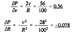
and so,

or,

about 5%. You will notice that apart from giving us an uncertainty estimate this analysis also shows that the likely error in our power measurement is almost entirely due to the uncertainty in resistance. To improve the accuracy we should therefore concentrate on reducing the uncertainty of the resistance measurement, not on improving the voltmeter. This kind of information can save a lot of time and money (voltmeters are expensive, resistors are not).

1. Holman J P, 2001, Experimental Methods for Engineers, 7th Edition, McGraw Hill, New York.
2. Kline S J and McClintock F A, 1953, "Describing Uncertainties in Single Sample Experiments", Mechanical Engineering, vol. 75, pp. 3.

-------------------------------------------------------------------------------------
        0       0.01    0.02    0.03    0.04    0.05    0.06    0.07    0.08    0.09
-------------------------------------------------------------------------------------
0.0     00000   00399   00798   01197   01595   01994   02392   02790   03188   03586
0.1     03983   04380   04776   05172   05567   05962   06356   06749   07142   07355
0.2     07926   08317   08706   09095   09483   09871   10257   10642   11026   11409
0.3     11791   12172   12552   12930   13307   13683   14058   14431   14803   15173
0.4     15554   15910   16276   16640   17003   17364   17724   18082   18439   18793
0.5     19146   19497   19847   20194   20450   20884   21226   21566   21904   22240
0.6     22575   22907   23237   23565   23891   24215   24537   24857   25175   25490
0.7     25804   26115   26424   26730   27035   27337   27637   27935   28230   28524
0.8     28814   29103   29389   29673   29955   30234   30511   30785   31057   31327
0.9     31594   31859   32121   32381   32639   32894   33147   33398   33646   33891
1.0     34134   34375   34614   34850   35083   35313   35543   35769   35993   36214
1.1     36433   36650   36864   37076   37286   37493   37698   37900   38100   38298
1.2     38493   38686   38877   39065   39251   39435   39617   39796   39973   40147
1.3     40320   40490   40658   40824   40988   41198   41308   41466   41621   41774
1.4     41924   42073   42220   42364   42507   42647   42786   42922   43056   43189
1.5     43319   43448   43574   43699   43822   43943   44062   44179   44295   44408
1.6     44520   44630   44738   44845   44950   45053   45154   45254   45352   45449
1.7     45543   45637   45728   45818   45907   45994   46080   46164   46246   46327
1.8     46407   46485   46562   46638   46712   46784   46856   46926   46995   47062
1.9     47128   47193   47257   47320   47381   47441   47500   47558   47615   47670
2.0     47725   47778   47831   47882   47932   47962   48030   48077   48124   48169
2.1     48214   48257   48300   48341   48382   48422   48461   48500   48537   48574
2.2     48610   48645   48679   48713   48745   48778   48809   48840   48870   48899
2.3     48928   48956   48983   49010   49036   49061   49086   49111   49134   49158
2.4     49180   49202   49224   49245   49266   49286   49305   49324   49343   49361
2.5     49379   49296   49413   49430   49446   49461   49477   49492   49506   49520
2.6     49534   49547   49560   49573   49585   49598   49609   49621   49632   49643
2.7     49653   49664   49674   49683   49693   49702   49711   49720   49728   49736
2.8     49744   49752   49760   49767   49774   49781   49788   49795   49801   49807
2.9     49813   49819   49825   49831   49836   49841   49846   49851   49856   49861
3.0     49865                                                                   
3.5     4997674
4.0     4999683
4.5     4999966
5.0     4999997133
-------------------------------------------------------------------------------------