Aurelien Borgoltz, William J. Devenport, Steven R. Edwards, and Brian Petrosky
Last revised 9 February 2019
Aerospace and Ocean Engineers use analog electronic instrumentation to set up, test, and calibrate measurement and control systems, whether or not those systems collect analog or digital data. These systems form an integral part of the development of modern aircraft and ships. Invariably such systems do not work without considerable effort from the engineer.
Consider setting up the measurement system shown in the figure. This could, for example, be for measuring the flow rate in a fuel line, for sensing the deformation in a ship structure or for determining flow speed past an aircraft or in a wind tunnel.
Setting up the sensor will typically involve measuring its resistance, for which we need a multimeter. It may be necessary to determine the dynamic response of the filter or sensor for which a function generator, frequency counter and oscilloscope are used. When the system does not work, the multimeter and oscilloscope may be used to check the connections between components and the output of individual components in the measurement system. To run the sensor, amplifier, and filter, a power supply may be needed. These devices are standard electronic test instruments used throughout all branches of engineering.
The objective of this lab is to teach you how to use standard instruments used in setting up the analog components of a measurement system. You will learn how to use a power supply, function generator, voltmeter and oscilloscope, and you will learn how to connect these devices together to make the measurement and control system used in Experiment 6. A short time may also be spent on installing LabView software on your computer, to be used later in the course.
The lab assumes that you have a basic knowledge of electronics, and some familiarity with Experiment 6. To prepare for this lab you should therefore
During the lab period you work in groups of two or three students to understand and use the instrumentation under the direction and guidance of an instructor. You are expected to take notes (electronic or on paper) to record your experiences. It is important you save your notes as you will need them to set up and perform Experiment 6 during the second lab period.
You will be given specific instructions during lab (copies of any materials will be made available on this page, linked from the left hand column). The material below gives a complete description of the instrumentation you will be using.
Power supplies are used to generate constant d.c. signals. These steady signals can be used to supply a measurement circuit or sensor with power or to calibrate an instrument. One of the power supplies used in the lab is the BK Precision Model 1673. It is typical of such devices. The power switch is located at the top left.
First we will learn how to set up the power supply to produce a constant voltage signal. Voltage is a relative quantity. To supply a voltage you therefore need two connectors. The only absolute reference for voltage is 'ground' - the voltage of planet earth.
The 1673 can simultaneously supply up to 3 different DC voltages from the 3 ports: the Master, Slave, and fixed output sources. Each port has 3 terminals, one red (+), one black (-), and one green (ground). The fixed output only has positive and negative outputs. The voltage difference between these terminals is the voltage supplied. The fixed port supplies a constant voltage of 5 V wuth a maximum current of 3A. The master and slave ports can supply any voltage between 0 and 32 volts with maximum current of 12A (each). The output of any of these ports may be made relative to ground by connecting either the red or black terminal to the green ground terminal.
2.1 Getting a 5 V signal.
To get a fixed 5 V signal from the power supply, you simply need to connect two
cables with 'banana' plug connectors to the '-' and '+' terminals of the fixed
port (see below).

When the power supply is turned on, the difference between the voltages of these terminals, and thus the far ends of the cables, will be 5 V. The cables thus deliver this voltage to whatever device you want. (Note that you can overload this system by connecting the two cables to a device that has little or no resistance, so that the 5 V would cause a really big current to flow. In that case the voltage supplied will drop to a level that the power supply can sustain - see the electronics review session discussion of 'internal resistance'.)
Now, the absolute level of the voltage of the two cables will be arbitrary and may float around (it is only the difference that is set at 5 V). If this is a problem, you can fix the voltage in one of two ways. First you can use an 3rd cable to connect the '-' terminal of the fixed port to ground, in which case then '+' terminal would now be at 5 V relative to ground. (Note that banana connectors can 'piggyback' on each other so that two cables can be connected to the '-' terminal.) Alternatively, you can connect the '+' terminal, in which case '-' terminal would be at -5 V relative to ground.
2.2 Getting a variable voltage.
Either of the adjustable master or slave ports can be used to get a variable voltage.
Both work in the same way as the fixed port. To set up the master to produce a voltage of 12 V
(relative to ground) you would connect the '-' terminal of port to the ground
terminal. Then you
would connect a second and third cable to the '+' and '-' terminals of the terminals on the right.
This second and third cables carry the voltage signal away from the power
supply.
To set the output voltage that will be delivered through these cables we would need to ensure that the master voltage and current control knobs are pushed in. Then turn the voltage control knob. The voltage setting is then indicated on the meters.
The meters are located in the center of the front panel. These indicate the output voltage and current of the master and slave supplies. To set 12 V, turn the voltage control knob from left to right for the master until the display reads 12 volts.
Note that the current control knob may not appear to do much here. In particular, if your output cables aren't connected to anything you will find that the current meter stubbornly reads zero however you turn the knob. This occurs because there is no way any current can flow out of the positive terminal and into the negative one unless there is a direct or indirect connection. So what is the current control for? To understand you must know how the power supply operates.
Most of the time the power supply ports operate as voltage sources. That is, they try to maintain the voltage set by the 'voltage control' knob regardless of the current flow needed to do this. Sometimes, however, it is not possible or desirable to have the terminals maintain the set voltage. Suppose you connected the positive and negative terminals directly together with a cable of near-zero resistance - such a large current would have to flow to maintain the voltage that it could destroy the unit. Alternatively, and more realistically, suppose you are supplying a voltage to a sensor. In this case, you would probably want a constant voltage but not if it means a large current that would destroy the sensor. For these reasons the power supply has current limiters. The limits for each port are set by the current control knobs from zero amps up to a maximum of 0.5 amps.
In summary, as long as the current is less than the limit, each port supplies the set voltage and whatever current is necessary to maintain it (like a voltage source). If the necessary current exceeds the limit then the port simply supplies the set current and whatever voltage is necessary (like a current source). In the latter case, the overload light will come on.
2.3 Other modes of operation
There are two other modes for using the master and slave supplies that may be selected using the master voltage control knob - 'parallel' and 'series'. In 'parallel' mode the voltage and current limit settings of the slave supply are always held to be the same as those of the master.
In this mode the slave controls do nothing.
In 'series' mode the '+' slave terminal is connected internally to the '-' master terminal. Both supplies are then used as a single power supply with the output taken between the '-' slave terminal and the '+' master terminal.
This power supply may be controlled by the master control knobs only. The reason for using series mode is that it doubles the available voltage. In series mode the output is double that indicated on the meter.
The three different output mode settings are summarized in the diagrams below:
Multimeters are used to measure resistance, voltage and current. This makes the multimeter one of the most important instruments. We use the BK Precision 2831 E in the lab. This is typical of such instruments. The power switch is again located on the upper left of the front panel.
The multimeter has three buttons indicated above that determine which type of measurement is being made. For example, if you wanted to measure the resistance of a transducer, you would select the resistance mode on the multimeter. Then you would connect the transducer to the multimeter by using cables and read the display. Likewise, current and voltage modes can easily be set.
3.1 Measuring a resistance
To measure resistance with the multimeter, you need to set the multimeter to the resistance mode
by pushing the 'W' button. Next, you need to attach cables to the multimeter ports. You may use any cable with
a banana connector on one end. You may want to pick cables that have a 'probe' connector
(metal spike) or an alligator clip (spring loaded clamp) at the other end, as
these are particularly useful for positioning on a contact, or clipping to a
wire.
Insert one cable into the red port on the front of the meter and another cable into the black port. The red port is used for resistance measurements. The black port provides a return path so that the resistance to be measured forms part of a circuit. It is called 'common' or COM. Note that it is not a ground.
Now connect the other ends of the cables to opposite ends of the resistor or component whose resistance you want to measure. (Note that any power to the component must be turned off, and at least one end must be disconnected from any other electronics if you want the resistance measurement to be meaningful.) You will see numbers appear on the multimeter display. If these numbers are all zero, then the range setting on the multimeter is too high and you should lower it. The ranges for the resistance mode of the multimeter are listed below the display ( as indicated by the yellow shading below).
If only the number 1 appears in the left most position, then the range setting is too low and the resistance value is 'out of range'. In this case, increase the range setting. If the display shows actual values, then this is the value of the resistor. Try out different range settings to see which one gives you the most precision. Remember to check your range setting before reading the display e.g. if the range setting is 20 K the display is in kOhms, if it is 20 M the display is in MOhms.
When measuring small resistances it is good practice to also connect the far ends of the cables (that you attached to the component) together and measure this resistance. This resistance (of the cables and connectors) should then be subtracted from your readings.
3.2 Measuring a voltage
Set the multimeter to the voltage mode by pressing in the 'VOLTS'
button. Insert one banana plug cable each into the red and black ports, and then the other
ends of the cables to the two sides of the component or two the two contacts
across which you want to measure the voltage. For a voltage you will
generally want the circuit containing the component of the contacts to be
powered up when you make your measurement. The range of the voltage measurement is determined by the buttons below the multimeter display
and over-range and under-range are indicated in the same way as for resistance
measurements. Note that to protect the instrument, you should always select
the highest range first when making measurements of unknown voltages.
There are two different types of voltage measurements. These are AC and DC. The button to the left of the voltage mode button toggles the multimeter from AC to DC. When making a voltage measurement in DC mode, the multimeter measures the time average voltage signal. In AC mode, the multimeter measures the R.M.S (root mean square) of the fluctuating part of the signal.
The RMS tells you how large the fluctuations in the signal are on average. Mathematically:
DC or average value:
AC or RMS value:
where, for periodic signals, T is the period. Note that for sinusoidal signals the RMS is 1/√2 times the amplitude A.
3.3 Measuring a current
The multimeter can also measure currents through a component or circuit element. Set the multimeter to the current mode
(the 'A' button). The white ports on the front of the multimeter are used to measure currents. The top port is unfused and can measure currents up to 10 A. The bottom port is used to measure small currents of 2 A or less and is fused.
Insert one banana plug cable to the white port that fits your expectations (use
the 10 A port if you are unsure how big the current will be) and another into the
black 'COM' port.
You need to connect the other ends of these cables to your circuit so that the current you want to measure actually passes into the white port and out of the black port. This means, for example, if you want to measure the current through a cable between two devices, you will have to disconnect that cable, and reconnect it through the meter.
The range settings, located below the multimeter display, work in the much the same way as they do for resistance and voltage measurements. Always select the highest range setting first when measuring unknown currents. Note that the meter will measure either in DC or AC mode depending on the setting of the left hand 'AC/DC' button, and thus displays either the time average or R.M.S. current (see the above discussion on voltages).
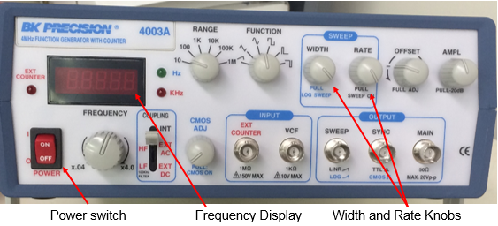
Often in Aerospace and Ocean Engineering applications, we need fluctuating signals to determine, for example, the dynamic response of sensors or systems. Such signals are produced by a function generator. The BK Precision 4003A used in instrumentation lab is a fairly standard function generator. This unit can be turned on using the power switch on the far left hand side. When using this instrument, make sure the WIDTH and RATE knobs are pushed in. We will not discuss these features. If you are interested, these SWEEP controls, along with the SYNC output, are described in the instrument handbook, which should be available in the lab.
4.1 Generating a Signal
The function generator can be used to produce six different kinds of signals: square
wave, triangular wave, ramp wave, and sine wave, positive pulse, and negative pulse.
The function knob determines the type of signal the instrument produces.
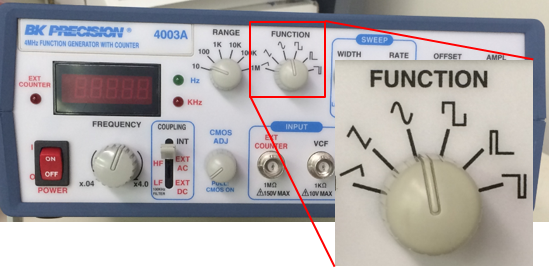
With the knob selecting sine-wave, a sine wave will be produced, for example. The function generator also has a range settings knob knob to determine the order of magnitude of the frequency generated. This knob is shown below.
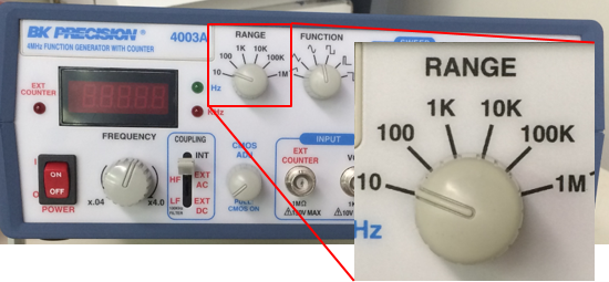
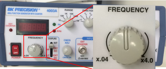
To set a frequency of 1 kHz, for example, you would need to move the RANGE knob to the �1K� option. To control the exact frequency of the signal, the frequency control knob (shown below) is used. This knob is used to adjust the frequency from 4% to 400% of its range setting. In this (1 kHz) example you would need to turn this control to the 1.0 position.
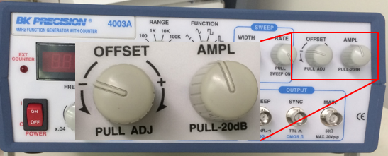
With the AMPL knob pulled out, the range is 0 - 2 V peak-to-peak, with it in it is 0 - 20 V peak-to-peak. Twist the knob left or right to control the exact peak-to-peak voltage. The peak-to-peak voltage is twice the amplitude. The amplitude control knob adjusts the amplitude from the minimum of the range (MIN) to the maximum (MAX).
Finally, we can control the DC offset of the signal, defined below.
Locate the DC offset control (to the left of the amplitude control). If this knob is pushed in then the DC offset is zero. If it is pulled out then the DC offset may be selected by turning the knob over a maximum range of -10 V (-) to +10 V (+). The actual range depends strongly on how the rest of the unit is set up. Note that there are no meters on this unit to show signal amplitude or DC offset. You must use the multimeter to determine the exact values set.
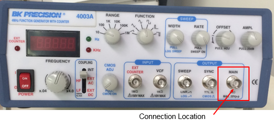
The signal from the function generator is output through the MAIN port (highlighted above). This port fits a BNC connector and coaxial cable.
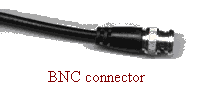
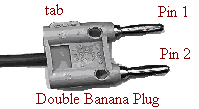
You will find coaxial cables near your station with a BNC connector on one end a double banana plug on the other (see right). The double banana plug fits into adjacent ports of the multimeter. Note that the coaxial cable has two conductors inside it - one connects the outer part of the BNC connector to pin 1 of the banana plug (identified by the tab on the side of the connector), the other connects the central pin of the BNC to pin 2.
The frequency counter is an instrument designed to measure the frequency of simple periodic signals, like sine waves. Such a measurement is often needed in diagnosing measurement system problems, or making measurements of periodic phenomena such as the resonant frequency of a structure. The Tektronix CFC250 counter used to be a feature in instrumentation labs and can measure the frequency of signals from 5 Hz to 100 MHz with amplitudes between 40 mV and 21 V. It is however becoming obsolete (as are most frequency counters), as other instruments (like oscilloscope or multimeter) can provide the same information.
5.1 Measuring a frequency
The counter has fairly simple controls. Signals are connected to the input port
on the bottom left of the front panel. The input port is designed to fit a BNC
cable, with a connector of the type shown below.

Such a BNC cable contains two conductors, one coaxial with the other. Once a signal is connected, its measured frequency appears on the display. If the frequency is too high, then the overrange light will come on and only the number 1 will appear on the left-hand side of the display. If the frequency is too low, or the measurement can't be made (non-periodic signal, signal too weak or too complicated), then a zero will appear on the right-hand side of the display.
If you don't get a satisfactory measurement the counter may need to be adjusted according to the magnitude of the signal being measured. The input voltage button switches the counter range between high voltage (3 - 42 V peak-to-peak) and low voltage (80 mV - 5 V peak-to-peak). Always use the high range first and then switch to the low range if the counter gives you no answer. Using the low range for a high-range signal will give you an answer but it may well be wrong.
The oscilloscope (or 'scope') is a device designed to display a voltage signal in visual form. Since in measurement systems we usually use voltage signals to represent the physical quantity we are measuring (e.g. strain, pressure, temperature), this makes the oscilloscope perhaps the most useful diagnostic instrument. The oscilloscope can also be used for some quantitative measurements, such as voltage amplitude and frequency (though not with nearly the accuracy of a multimeter or counter), and can be used to compare two separate signals and estimate their relative characteristics (such as the phase lag between them). The scope used most often in lab, the Tektronix TBS 1052B, is typical in design and features.
6.1 Basic Set Up
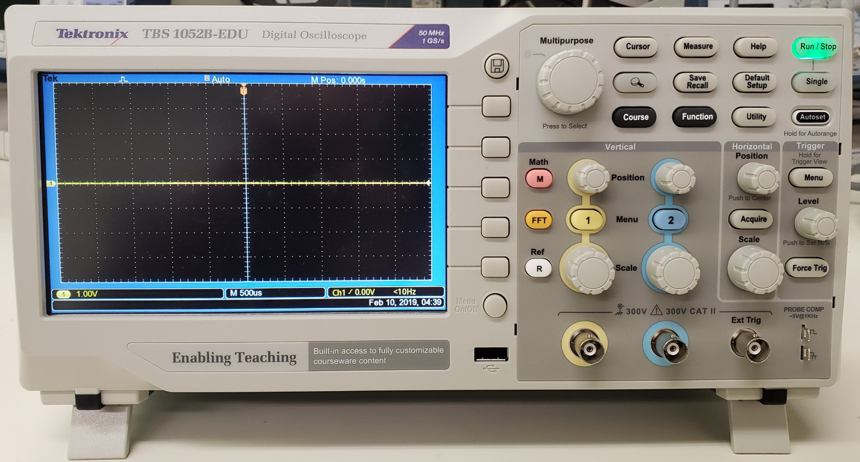
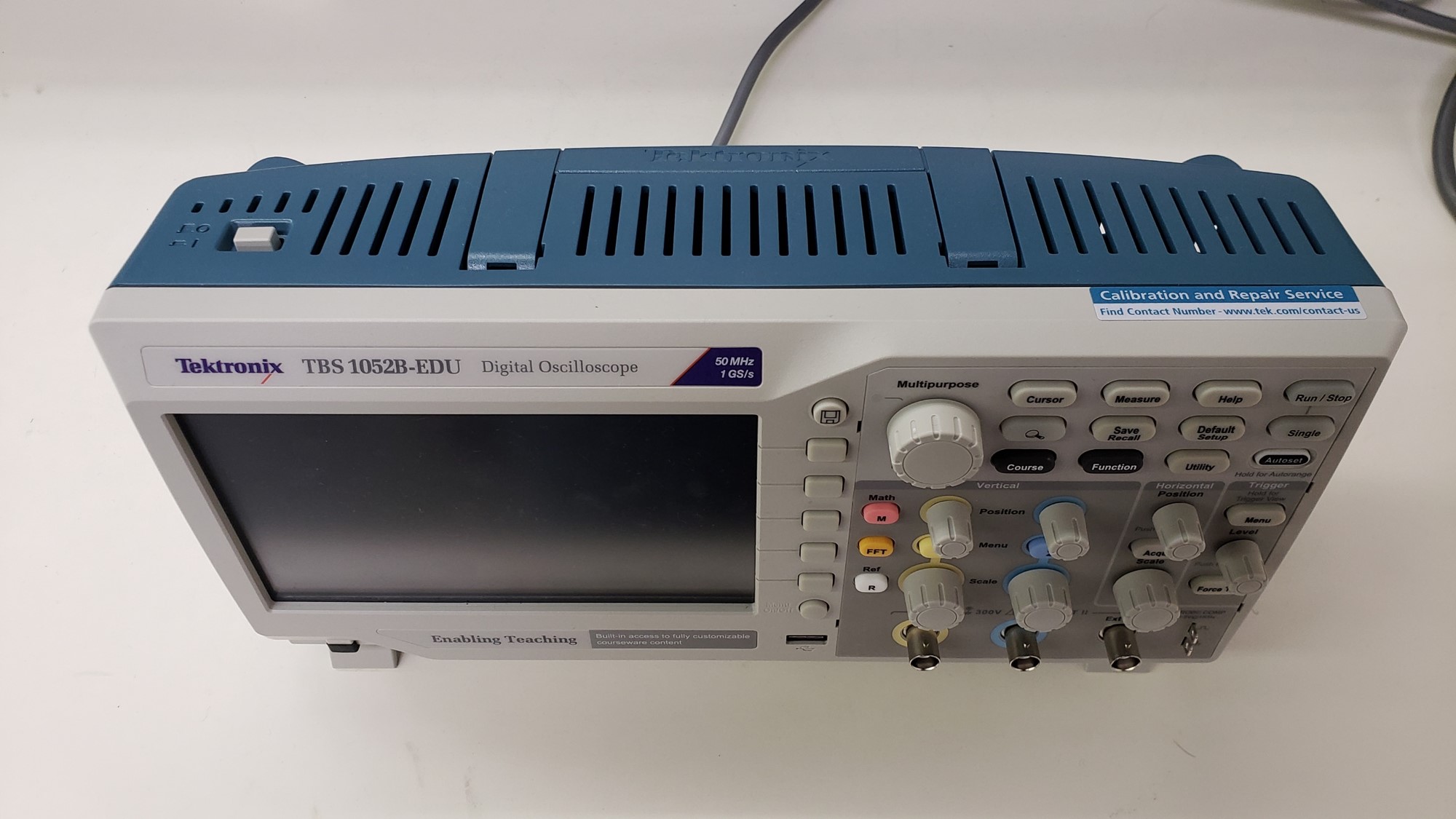
The oscilloscope is turned on using the power button (indicated below). After a
few seconds a horizontal line should appear on the screen. If this is your first
time using the scope and a line doesn't appear ask your lab instructor to help.
The line, called a 'trace' is a plot of voltage (on the vertical scale) against time (on the horizontal scale). The line will be flat when no voltage signal is connected to the scope.
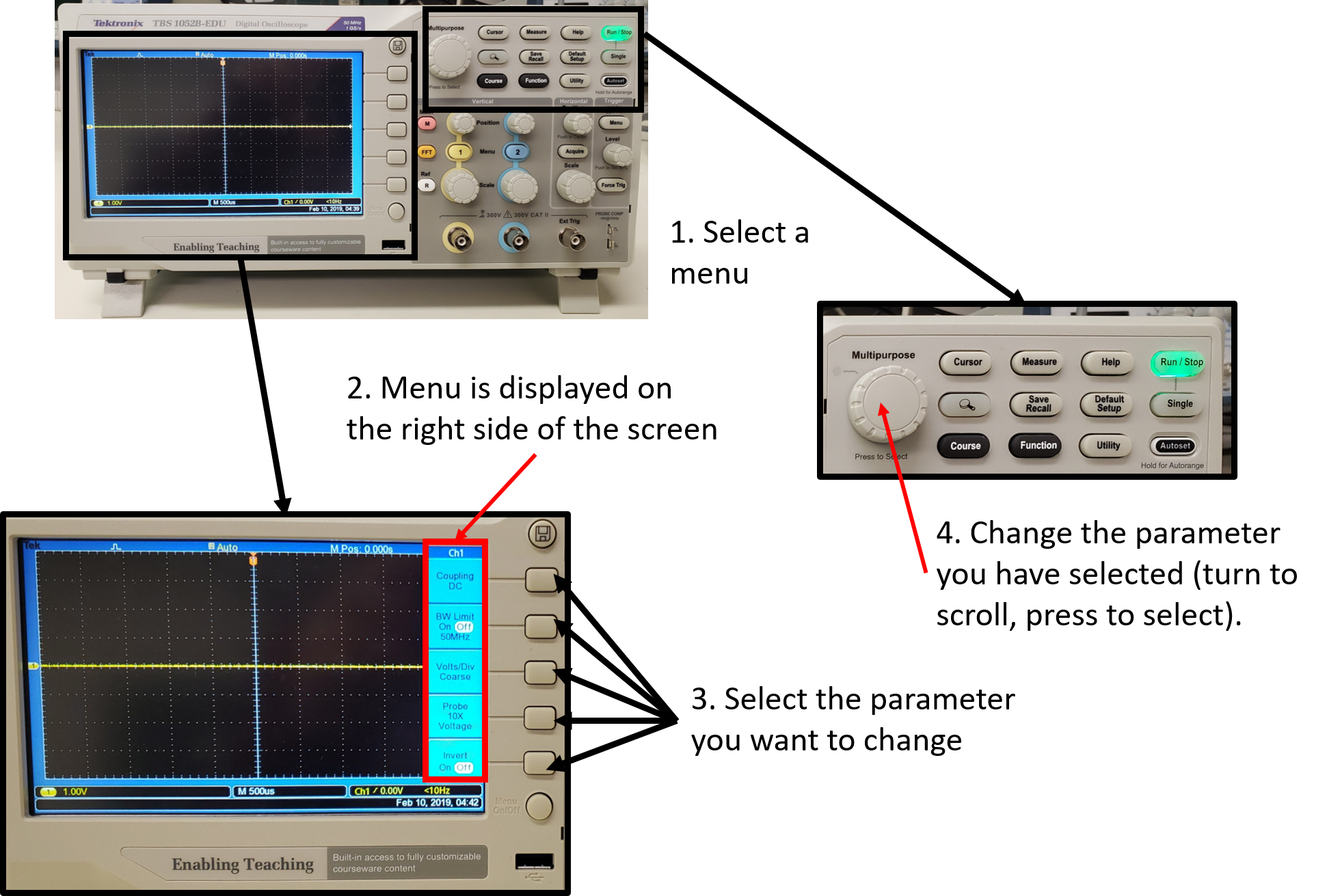
The TBS 1052B is a digital oscilloscope that functions very much like a computer. Most of the settings can be changed through various menus accessible from the top control panel:
You may alter the appearance of the trace using the DISPLAY menu indicated in the figure. Turn these to get a feel for what they do. Set them to give a sharp, clearly visible trace. Note that it is not a good idea to use a higher intensity setting than is needed since this will tend to wear out the scope and screen.
Note that the oscilloscope screen has graduations (or 'divisions'). This is to enable you to make quantitative measurements of signals displayed. You can also try the MEASURE and CURSOR menus. The MEASURE menu allows you to measure various quantities (frequency, mean, peak-to-peak, etc...) for one or two channels. The CURSOR menu uses two lines to measure any feature on the vertical or horizontal axes. Try these out for yourself.
The scope has many controls and so can be confusing, especially if the previous user left them in an unusual configuration. The following is a set of instructions that places the scope in a 'normal' initial state with a signal showing. Descriptions of the individual controls referred to hear are given later in this section.
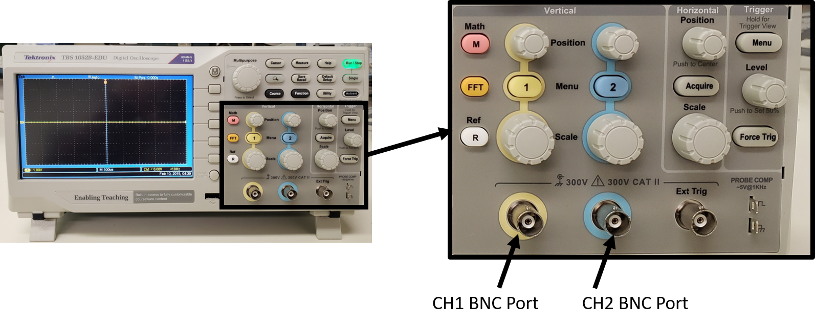
Signals are connected to the scope through one of two BNC sockets, located as shown above. These accept cables with connectors of the type shown below.
There are two sockets, because the scope can simultaneously display up to two signals. The signals and connectors are identified as CH 1 and CH 2, for channels 1 and 2. Note that the signal is actually provided to the scope through the central pin of the BNC sockets. The outer shield is a ground connection (not just a common) so you must be a little careful what you connect to it. (E.g. if you set the power supply to provide 5V relative to ground and then connect the 5V to the BNC shield the resulting mismatch might cause problems the scope.)
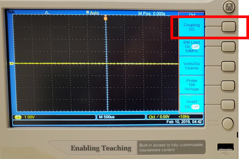
In the CH 1 MENU , you will find the Coupling value that controls the way in which the signal is connected to the scope. By moving this switch you can choose 'DC', 'AC', or 'GND'. When DC is selected, the whole signal (mean + fluctuating parts) is connected to the scope and (if set up appropriately) displayed. With AC selected only the fluctuating part is connected. With GND (or ground) the signal is disconnected and the position of the trace corresponding to zero volts will be displayed on the screen.
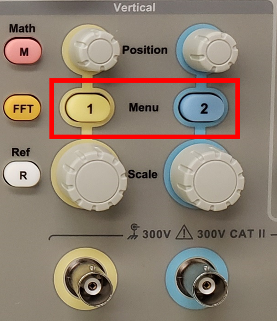
When you have made your connections, you need to tell the oscilloscope what to display using the CH 1 MENU and CH 2 MENU buttons. Pressing these buttons will toggle the display of their respective channel. Channel 1 signal appears as a yellow trace, while Channel 2 signal is blue. It is therefore possible to display the signals from both channels at the same time.
The MATH MENU button can be used to display an arithmetic combination of two signals. You can select from addition, substraction, multiplication, addition or Fourier Transform (FFT). The resulting signal is plotted in red.
6.3 Setting the Vertical Scale
Scopes give you the same control over displaying a signal as you would have
over plotting it on a piece of graph paper. You can independently control the
origin and the scale of the voltage displayed on the vertical axis. There are
duplicate controls for the two channels.
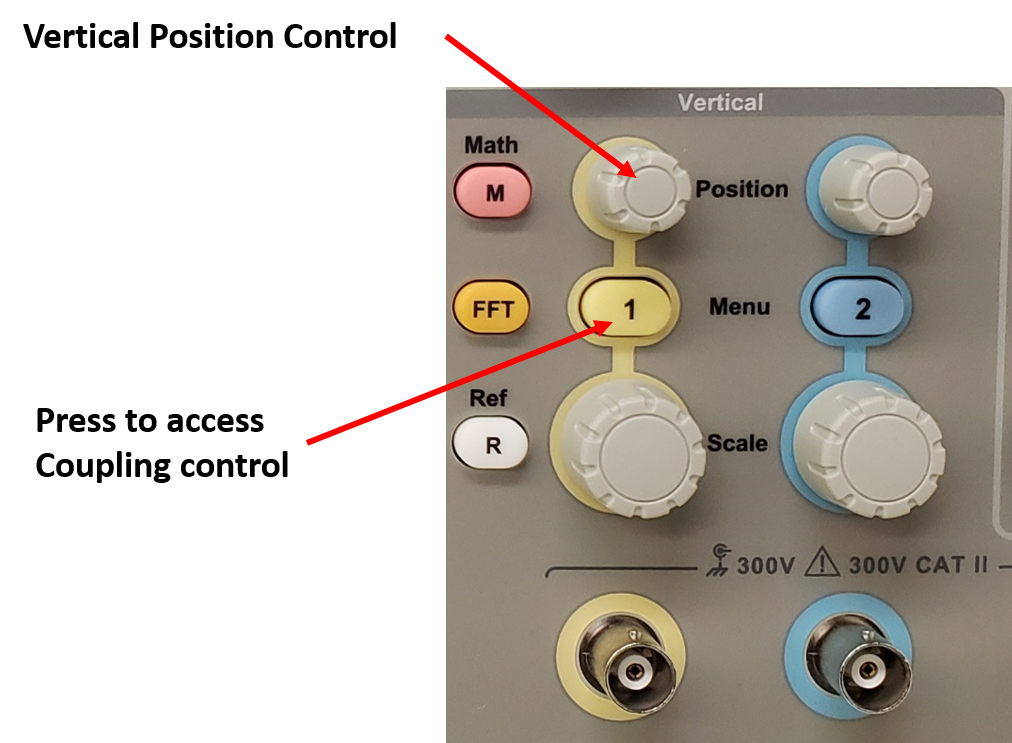
The vertical 'POSITION' controls are used to set the origin. Turning the POSITION control for CH1 for examples simply moves the signal up and down on the screen (i.e. the origin is moving up and down). If your objective is to make an absolute voltage measurement (rather than just look at the form of the signal) you will want to know quantitatively where the origin you've set is. You can do this by selecting GND coupling to plot zero volts on the screen.
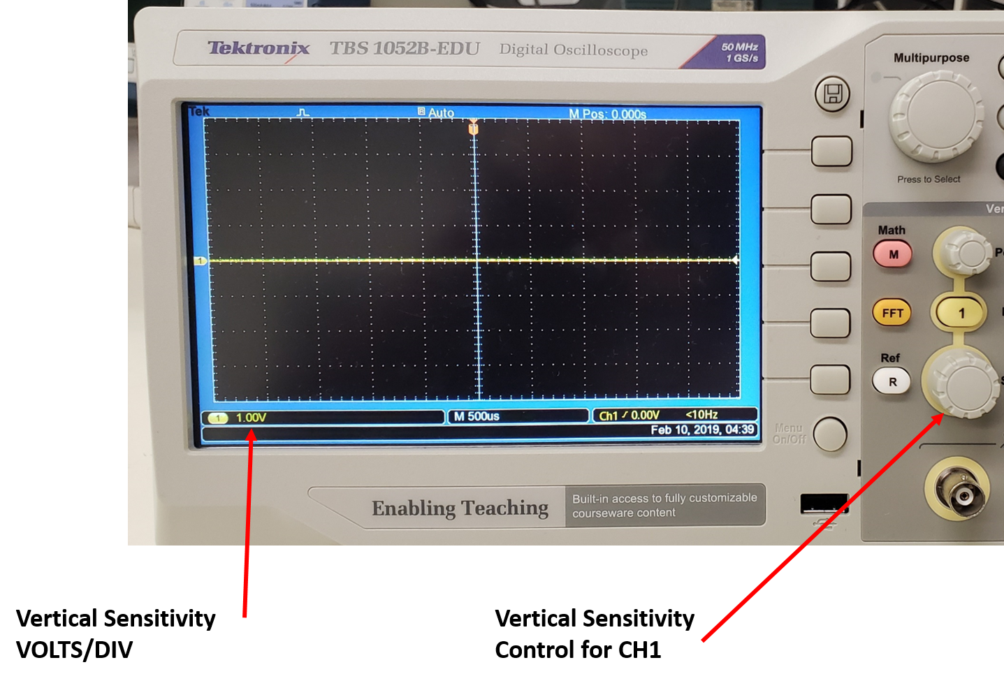
For controlling the scale of the voltage axis there is a VOLTS/DIV control. This sets the voltage represented by each of the large vertical divisions on the screen. The actual value set is indicated by the number in ther lower left corner of the screen and may be varied from 5 mV per division to 5 V per division.
If you need finer resolution in the increments of VOLTS/DIV you can press the CH 1 MENU and change Volts/Div from Coarse to Fine.
Note that it is perfectly possible to set the POSITION and/or VOLTS/DIV control so that the signal you want to look at, or even the voltage origin, is off the screen so that you see no trace. If you think this has happened the best way to get your signal back is to increase the VOLTS/DIV setting, and then to rotate POSITION knob until the trace appears.
6.4 Setting the Horizontal Scale
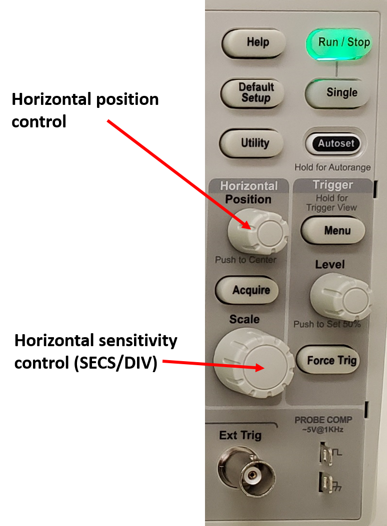
The controls for the horizontal (time) axis are located as shown in the picture. The same horizontal scale is used for both channels, so there is only one set of controls. For controlling the time origin (i.e. for moving the signal horizontally across the screen) there is a POSITION control. For controlling the scale of the time axis there is a knob labeled 'SEC/DIV'. This sets the time represented by each of the large horizontal divisions on the screen. The actual value set is indicated at the bottom of the screen (just above the date) and may be varied from 5 nanoseconds per division to 50 seconds per division.
6.5 Getting a Steady Display
The scope provides a continuous display of a signal by repeatedly re-drawing
the trace (the trace is actually generated by an electron beam that is swept
across the display at a constant rate). When viewing a periodic signal it is
unlikely that the scope will start redrawing the trace at the same point in the
waveform every time, unless we set it to do that. The results can be an unsteady
jumble of overlaid traces, or image of the signal that drifts to the left or
right with time (possibly quite fast).
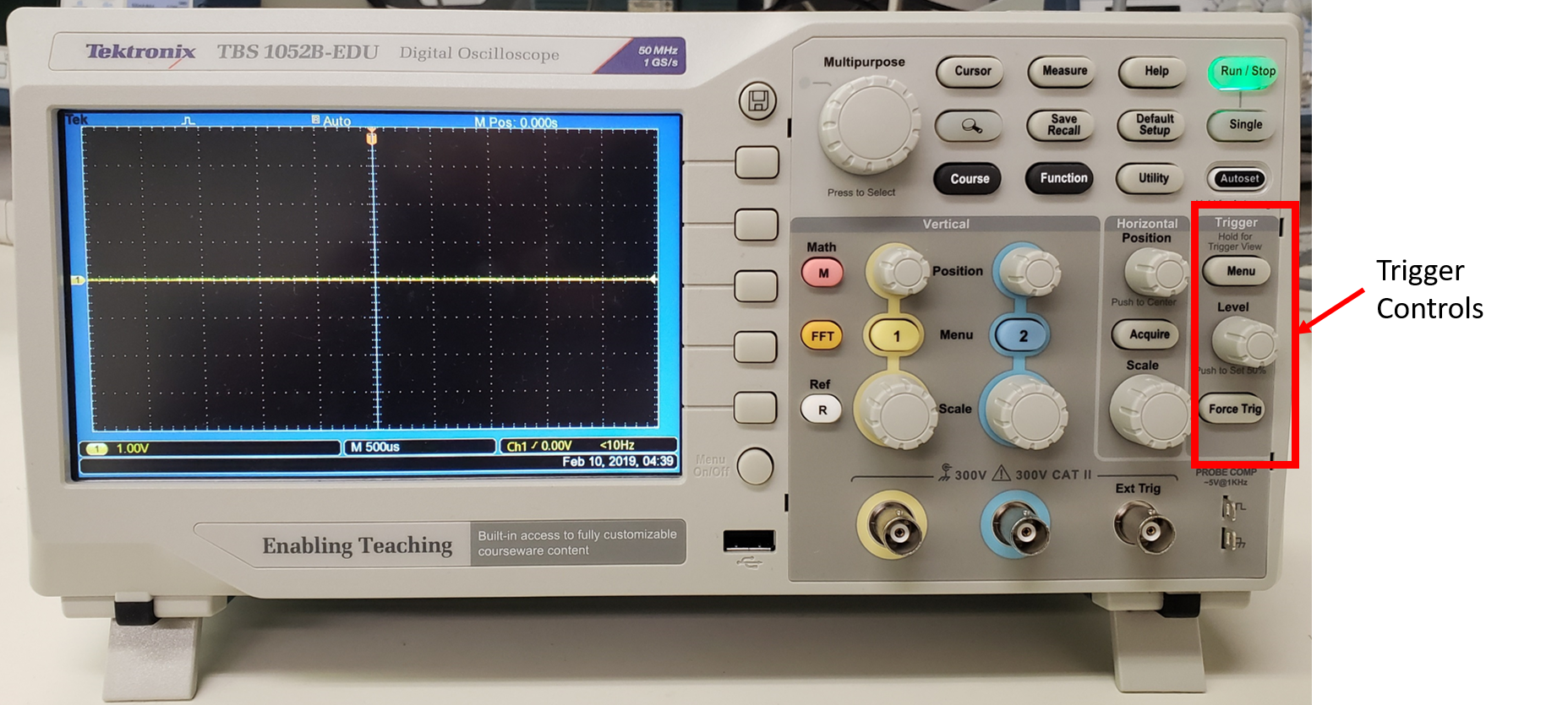
To set the scope to display a steady image of a periodic signal we use the TRIGGER controls. The 'trigger' is the condition under which the scope begins drawing the trace. The scope determines this condition by comparing a signal (which may or may not be that displayed) with some preset criteria. You can control the signal and the criteria. You can also control the mode - how the trigger decision is made.
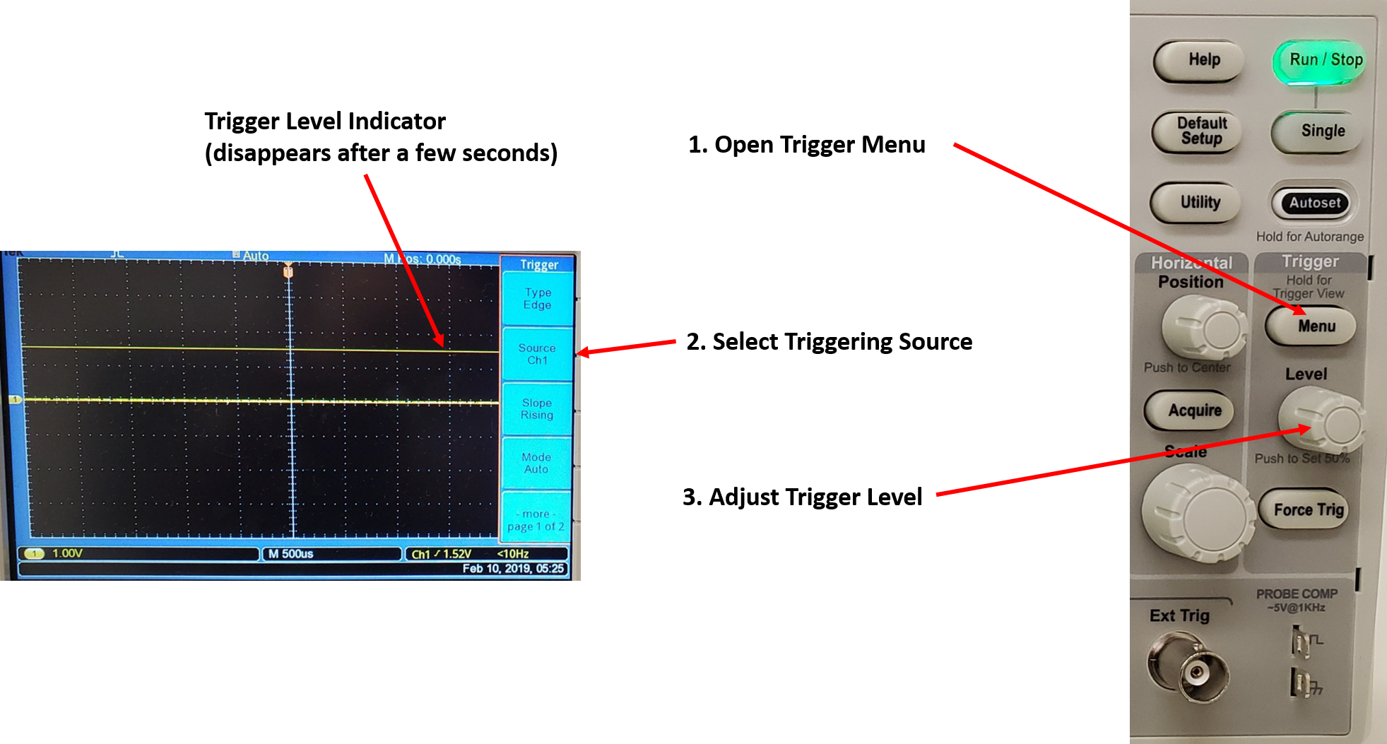
To control the source of the signal used to trigger the scope the TRIG MENU is used . The selecting button allows you to choose from CH1 or CH2 (in which case the scope will trigger off one of the input signals), EXT, EXT/5, or AC Line. If EXT or EXT/5 is selected the scope triggers off a separate signal altogether, which you provide to the scope through the BNC socket located just below the Horizontal SEC/DIV control. If AC Line is selected, the scope will trigger off the 115V 60Hz mains power at 60 times per second.
Once you have selected the source of the signal you can select the criteria under which triggering will occur. Triggering occurs when the selected signal crosses a threshold voltage, which you can set using the LEVEL knob. The SLOPE feature in the TRIG MENU to the left of this allows you to select rising or falling which, respectively, determine whether the scope triggers as the voltage rises through the trigger level or as it falls through it.
6.6 Measuring Phase
Since the scope can be set up to display two signals simultaneously, it is
possible to use it to measure the phase lag between those two signals.
Phase difference is the time delay between two signals expressed as
an angle. Consider the example shown in the figure. Assuming the time
delay is less than one period then the phase difference in degrees is given by
360Dt/T, where Dt
is the time delay between the signals and T the period . A basic
phase measurement can thus be made by simultaneously displaying two signals together on the screen
(see connecting signals), and using the horizontal scale and
the SEC/DIV setting to measure the time delay and period.
Quite often we are particularly interested not in the phase lag itself, but being able to identify when it is 90 degrees. This is because many simple dynamical systems have a phase lag between excitation and response of 90 degrees at their resonant frequency. A phase lag of 90 degrees is most easily recognized by using the scope in X-Y mode.
XY mode is selected by turning opening the DISPLAY menu and changing Format from "YT" to "XY" as shown below. Note that you will need to adjust the time sensitivity to get the Lissajou plot to display properly.
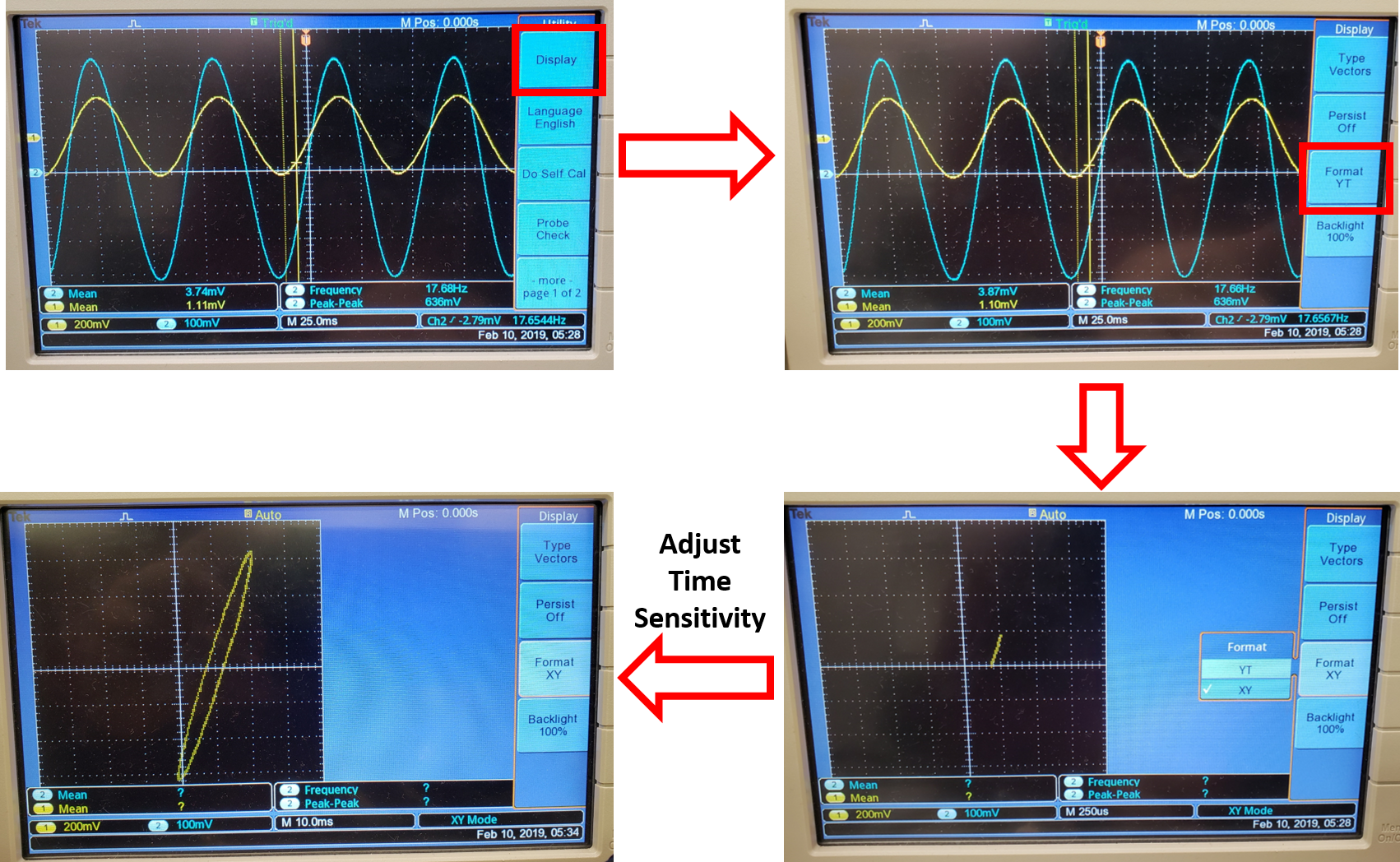
In this mode the scope shows a single trace generated by plotting the channel 1 voltage on the horizontal axis against channel 2 on the vertical axis. The VOLTS/DIV and position controls for channels 1 and 2 still work in exactly the same way, except the channel 1 controls now determine the horizontal axis scale and position.
If two signals of the same frequency are connected to channels 1 and 2 in this mode, the result is usually a closed loop of some kind, called a Lissajous figure. If the signals are of slightly different frequency the loop will rotate, the speed of rotation increasing with the difference in. frequency. If the two signals are sine waves of the same frequency, then very specific patterns are seen. If the signals are exactly in phase or 180 degrees out of phase, then you will see a straight line (see figure). If they are 90 degrees out of phase then you will see an ellipse with vertical and horizontal major and minor axes, thus this condition is easily recognized. If the phase angle is somewhere in between then it may be determined by the method shown in the figure.
6.7 When No Signal Appears...
Here are some quick fix tips for finding your signal.
Turn the VOLTS/DIV knobs to their maximum setting and the
vertical and horizontal POSITION knobs to the middle of their
range. Make sure that you are displaying the correct input
channel. Choose AC coupling for the input channel you are
using. Check to see that the Contrast is turned up. Press the AUTORANGE button (this will adjust the VOLTS/DIV and SEC/DIV automatically.
The scope will greatly shrink both the vertical and horizontal scales so that, if the signal was off the
screen, you will now see in which direction. Don't get too
exasperated. It is common to see even the most seasoned
professional fumbling around in embarrassed confusion for that
signal which would be SO good, if only you could see it...
6.8 Exercises
You will need to have read and understood how to use the
function generator before attempting these exercises.
1. Use the oscilloscope to display the a 1 V amplitude, 0 V offset, 100 Hz sine wave produced by the function generator. (You can get an amplitude of about 1 V by depressing the 0-2 V peak-to-peak button and turning the amplitude to MAX on the function generator.). Connect the signal to the CH1 input of the scope and select AC coupling. Set the remaining controls according to settings recommended for basic set up. Once you have the signal on the screen, verify the amplitude (by looking at the number of vertical divisions it covers), and the frequency (by looking at the number of horizontal divisions in one period).
2. After setting up the scope for exercise 1, try the following: