This laboratory is designed to

1. give you hands on experience of the smoke flow visualization technique, and
2. provide you with an opportunity to use this technique to study several wind tunnel flows.

An example of such visualization is provided in the video below (in the MP4 format) that was produced with a high-speed camera (courtesy of Dr. Todd Lowe and his student Brian Petrosky) in the smoke flow wind tunnel you will be using in your lab (using the airfoil model you can use in your experiment). The video has been processed to maximize contrast (which explains why the airfoil model is not visible at the center of the frame) to highligh the vorticular structures shedding from the leading and trailing edges.

You will be able to use this technique in a small smoke tunnel to study a number of flows, including particularly the flow past a stalled airfoil. Generating a flow in a wind tunnel that accurately models the flow over a real vehicle or vehicle component can be a lot harder than just having a model the right shape. During the course of this laboratory you will be able to investigate some of these problems. In particular you will be able to examine:

Reynolds number effects:  For an airfoil Reynolds number is usually defined as  where  is the free stream velocity, c the wing chord and the kinematic viscosity. It represents the typical ratio of the scale of inertial forces to that of viscous forces in the flow. Most engineering devices operate at large Reynolds numbers. A airplane wing with a chord length of 7ft, flying at 150 km/hr at sea level has a Reynolds number of 5,700,000. A hydroplane 1m in chord traveling at 35 knots (18 m/s) has a Reynolds number of 19,400,000. Reproducing such Reynolds numbers in a wind tunnel with a small model (say 0.25m chord) is usually not possible. Much wind tunnel work therefore relies on the assumption that flows remain largely unaltered by increase in Reynolds number. This is not always the case.

Blockage effects:  Blockage may occur as a result of the solid walls of a test section constraining the flow as it moves around a model. This constraint, which does not occur in free flight, increases the velocity of the flow as it passes the model, altering the flow pattern and characteristics. In the case of an airfoil, solid blockage tends to make the flow over an airfoil stall earlier than it otherwise would. This is because boundary layer separation occurs when in regions where the flow is decelerating, i.e. there is an adverse pressure gradient. The stronger the gradient the sooner separation will occur. Blockage increases the magnitude of the deceleration and thus the adverse pressure gradient produced by an airfoil. Interestingly, the reverse effect occurs in an open-jet wind tunnel. Here the wind-tunnel 'wall' is formed by the edge of the jet, and thus it can be deformed by the flow over the model. This deformation tends to reduce the magnitude of the accelerations and declarations experienced over the model.

A. Instrumentation for measuring the properties of the air.
The wind tunnel you will be given to use in this experiment uses the laboratory atmosphere as the working fluid. The properties of the air in the lab vary depending on the weather so it is important that at some stage in your experiment that you measure them, so you know what fluid you are working with. From the point of view of the dynamics of the air, the important properties are its density and viscosity (think of Bernoulli's equation and the Reynolds number).

Rather than measuring density directly, it is best obtained by measuring pressure and temperature and then using the equation of state for a perfect gas. You will obtain the atmospheric pressure by correcting the reading provided by the Blacksburg Airport Weather Station. The airport reports the current atmospheric pressure setting required to calibrate the altimeters in aircrafts. Therefore the value provided by the airport weather station is the sea-level value. The script below will convert the sea-level reading from the airport to the current atmospheric in Blacksburg (650m above sea level). Readings are provided with 1mbar uncertainty.

A digital thermometer (CNMC Model DBT0100T, shown in Figure 1, and typically located on top of the smoke tunnel inlet) for measuring atmospheric temperature is also present. The thermometer provides temperature with an uncertainty of 0.2℃ while also providing barometric pressure in mm of mercury (with an uncertainty of 0.375mmHg). The gas constant R in the equation of state for a perfect gas (p =RT) is 287 J/kg/K.

The temperature can also be used to infer the dynamic viscosity of the air using Sutherland's relation. For SI units,

B. Smoke flow visualization wind tunnel and equipment
A small horizontal smoke tunnel (Figure 2) will be at your disposal. The tunnel is an open-circuit design built by Aerolab (Laurel, MD) and powered by a small 1/5HP constant speed electric compressor (Whisper Aire WAC1000). The compressor located at the exit of the circuit pulls air from the room into the test section through a honeycomb flow straightener (Figure 3). The wind tunnel inlet measures 30.5cm x 24.4cm. The flow straightener is made of hexagonal honeycomb, 17.8cm long with a cell size of 0.32cm. Atfer the honeycomb straightener, the flow passes through a 9.25:1 contraction before entering the test section. The test section (where the various models are mounted) is 27.8cm long and has a rectangular cross-section (25.4cm x 3.2cm). The honeycomb and high contraction ratio are paramount to produce laminar flow (a key requirement to ensure the visibility of the smoke filaments). Without these devices, any turbulence present in the flow would mix and diffuse the smoke. The flow exits the test section through a second set of honeycomb to further ensure a laminar flow.

The flow speed in the tunnel is regulated by a valve located at the outlet of the compressor. A knob located on the main control panel is used to open or close the valve. Turning the knob counterclockwise will increase the flow speed, clockwise will slow it down. The freestream velocity is monitored using a pressure tap located at the entrance of the test-section. The tap is connected to a Dwyer Series DM-1102 differential pressure gage mounted on the wind tunnel structure that measures the difference between the static pressure in the test-section and the atmospheric. The pressure gage has a maximum range of 0.25" W.C. with a resolution of +/-2% full scale. The flow velocity coming out of the contraction can then be found using Bernoulli's equation, p_o = p + ½ρU².

The "smoke", which is vaporized water, is produced by an ultrasonic water atomizer (Ocean Mist Mist Maker DK9 Series) shown in Figure 3. The resulting vapor is injected in the test section through a rake located 14.3cm upstream. The rake produces streaklines that are spaced 6.4mm apart. During operation, it is possible that water dropplets will accumulate on the rake and prevent the smoke injection. Pressing the PURGE button on the main control panel will provide a short blast of air to clear the rake.

During operation, the atomizer will get HOT in approximately 15min. Turn off the tunnel and allow the reservoir to cool if needed. Avoid contact with the reservoir.

 The tunnel comes with some additional supplies and equipment including,

1. Several models are available (some of which can be used with an auxiliary blower or a spin motor).
   - a rectangular wing (Figure 4)
   - a delta wing (Figure 5)
   - a circular cylinder* (Figure 6)
   - a 25mm-diamater smooth sphere(Figure 7)
   - a 25mm-diameter sphere with dimples (Figure 8)
   - a series of 4 Clark-Y airfoils with a tangential blowing orifices, and various flap deflection angles (the flap length is 20% chord, and deflections are 0, 5, 10,and 15°)⁺ (Figure 9 through Figure 11)
   * The cylinder model can be connected to a spin motor located on the back of the tunnnel. What is the advantage of being able to test a spinning cylinder?
   When using the spin motor, be sure to engage the model all the way down the shaft as shown in Figure 7. DO NOT FORCE the model onto the shaft.
   ⁺ These models can be used with an auxiliary pump located on the back of the tunnnel. The pump can be used for suction and blowing (by swapping the hose connection) through the various models. What does blowing/suction accomplish in terms of airfoil performance?
2. Also provided are calipers, a metal ruler and tape measure so you can measure the model and wind tunnel dimensions and a overhead projector pen that can be used to temporarily used to mark the wind tunnel window if you desire.
3. Digital camera and tripod

A. Getting familiar with the equipment
    The following procedures are designed to help you get a feel for the smoke tunnel, its models and peripheral equipment. It is important that everybody get a hands on feel of how to use the apparatus and what its capabilities and problems are. Feel free to play with the apparatus at this stage, but don't forget to record your impressions in the logbook.

• Try out the barometer and thermometer and make initial readings. Try calculating the atmospheric density and viscosity, are the results sensible? Make estimates of the uncertainty in these primary measurements.
• Plug in the tunnel power chord. Turn on the test-section lights and the fan. Familiarize yourself with the tunnel control and make sure air flows through the circuit.
• Check the water level in the atomizer. If it's too low, ask your TA for TAP water. Once you press the SMOKE button on the Main Control Panel, the vapor should be produce within a minute or so. If nothing happens, ask your TA for assistance.
• While the tunnel is warming up set up the digital camera (your TA will show you how if you need help). Try out the camera. Try taking photos, and transferring them to your electronic logbook. (You could take some photos of the apparatus  to use in your report.) Photos of the smoke streams tend to be better when taken with the lights in the immediate vicinity of the tunnel turned off. Try setting up the camera on the tripod as close to the test section window as you can. Having the camera on the tripod, and thus in the same position for every photo can be very useful if later you want to quantitatively compare photos made at different conditions.
• When the smoke starts coming, take off the test section window and insert a model. Replace the window and look at the flow. Press the PURGE button if you need to clear any of the smoke holes. Try a photo - with flash, without, what's best? Figure 12 is a satisfactory sample picture.
• Try different models to see what the flow is like. Try varying the speed (i.e. Reynolds number) with each model and see what happens. Can you evaluate the speed of the flow in the test-section? The airfoil is a particularly interesting model since you can change the angle of attack (line the trailing edge up with the marks on the back of the test section). As you check out these flows, make a list in the logbook of important things to do/measure when you run the real test. E.g., measure the model (which dimensions?), measure where it is in the test section, how far from the strut, record the motor speed, take photo always from same position, don't forget the properties of the air, etc. If you are using the airfoil, what do you think the uncertainty on angle of attack is? If you are using another model what is you feeling about the accuracy with which you can position it?
• Try making a list in the logbook of any problems with the apparatus that you think might affect the quality of your results. A good way of judging the flow quality is to look at the smoke flow pattern with no model. Try sliding the smoke strut back and forth to visualize the whole flow, varying the speed. Do you see any imperfections? Do the imperfections change with speed? Are they worth documenting (this may depend on the goals you choose)?
• Try putting in the venturi to reduce the test section width - what's the quality of the flow with this? Do you think this will be useful for studying blockage effects?

Goal 1. Design, conduct and document a sequence of tests to determine the location of separation on one of the airfoils as a function of angle of attack at a fixed Reynolds number, and to assess wind tunnel effects that may have influenced your results.
Suggestions: Don't forget to look at the lists you generated above. For wind tunnel effects, you might try documenting the empty test section flow at the same condition. Maybe you can measure separation location more accurately directly off the wind tunnel window? Don't forget to document how accurately it can be measured. Try using blowing/suction, flaps. How do these devices affect the flow? Which one is most efficient? Try plotting separation location (x/c) vs. angle of attack in your electronic lab book as you go. If there are strange points in the curve, it maybe worth measuring them again.
Analysis suggestions for later.  Compute your best estimate of the Reynolds number and its uncertainty. Add error bars to your plots of stall location. For assessing wind tunnel effects, you could measure off streamline positions at the bottom of the wind tunnel window, with and without model and the modified test section window. A plot of these positions may help you distinguish wind-tunnel effects from other effects. Labeling pictures to indicate the significant features of each flow, and the significant imperfections of the wind tunnel flow will support any discussion you want to make in your report. 

Goal 2. Design, conduct and document a sequence of tests to take careful flow visualization pictures of a range of flows you have discussed previously in AOE 3014 at a fixed Reynolds number (like the flow over a cylinder), and to assess how wind tunnel effects may have influenced your results. (This would make a nice report later, where you can contrast what the pictures show with your expectations from the earlier course, referencing the text book.) What can the spin motor help you achieve in that case?
Suggestions: Don't forget your lists of things to measure in a real test - careful documentation of each flow will greatly enhance the value of your results. Choose a Reynolds number where you get good pictures. See suggestions above on wind tunnel effects. Be sure to record your impressions of each flow in the electronic log book as you see the flows, what was expected and what was not, you can see much more now than you will be able to observe later in a photo.
Analysis suggestions for later.  Compute your best estimate of the Reynolds number and its uncertainty. Label pictures to indicate the significant features of each flow, and the significant imperfections of the wind tunnel flow - this will support any discussion you want to make in your report. Make or copy (give a proper reference) figures showing the form of these flows as you were introduced to them in AOE 3014. Consider a quantitative comparison with theory. E.g. you could compare streamlines in the flow past the circular cylinder with actual calculations based on 2D potential flow theory. Show the theoretical and experimental results side-by-side, or over top of each other. Include details of the theoretical calculation in your report.

Goal 3. Choose a model flow. Design, conduct and document a sequence of tests to examine the effect of Reynolds number upon that model flow, and assess the extent to which wind tunnel effects may have influenced your results (this would include performing a calibration of the facility to accurately determine the flow speed).
Suggestions: You may wish to run a preliminary test to see if there is a model flow that has a greater Reynolds number dependence, as that would be easier to study. You will also need to find a way to evaluate the Reynolds number. Try to think of practical ways to do this (you could use a stopwatch, a digital camera etc...be creative). Can you trust the readings from the pressure gage? Can you take the resolution of the pressure gage as your primary uncertainty or do you see large fluctuations? Having the camera fixed on the tripod may be critical here in usefully comparing photos taken at different speeds, and without the model (at different speeds), as effects may be small. Try plotting significant features of the flow, e.g. separation location, tip vortex position, vs. Reynolds number as you go. If there are strange points on the curve, consider going back and re-measuring.
Analysis suggestions for later.  Compute your best estimate of the Reynolds numbers and their uncertainty. Add error bars to your plots showing the locations of significant features vs. Reynolds number. For assessing Reynolds number effects associated with the wind tunnel alone, you could measure off streamline positions at the bottom of the wind tunnel window, with and without model, and plot them against Reynolds number. Labeling pictures to indicate the significant features of each flow, and the significant imperfections of the wind tunnel flow will support the discussion you make in your report. Don't forget that you can also discuss the effects of Reynolds number upon the flow visualization technique itself - e.g. you could measure of the width of a representative smoke stream at the top of the test section window, with no model, vs. Reynolds number. Plotting this would then show the change in diffusion rate of the smoke as speed is increased.

Before starting your report please read all of Appendix 1. Check out the report grade sheet for this experiment, available in Appendix 1.

Title page
As detailed in Appendix 1.

Introduction
State logical objectives that best fit how your particular investigation turned out and what you actually discovered and learned in this experiment (no points for recycling the lab manual objectives). Then summarize what was done to achieve them. Follow this with a background to the technical area of the test and/or the techniques (e.g. the fluid dynamics and/or the experimental techniques you are using). This material can be drawn from the manual (no copying), classes, textbooks from prior courses, references cited in this chapter or even better, other sources you have tracked down yourself.  Finish with a summary of the layout of the rest of the report.

Apparatus and Instrumentation
 It is probably easiest to begin by describing the smoke tunnel itself. Include a diagram or labeled photo of the tunnel. Describe the figure in the text of the report including all the details that may be important to the flow it produces (e.g. open circuit, contraction ratio, dimensions and shape of the test section, type of vapor used, method of vapor production, method used to introduce vapor to the flow, location of smoke strut, flow speed uncertainty etc.). Next describe the model(s) you used. Diagrams or photos will be needed. Give the model dimensions (span, chord, diameter, airfoil shape designation) and location(s) that the models were placed in the test section (with the airfoil you should also include the chordwise location about which it was rotated to angle of attack). Don't forget to mention imperfections in the models and any uncertainties. Now mention the techniques used to make the measurements. Include in particular the digital camera, tripod and location. If you measured positions directly off the wind tunnel window, talk about how that was done (and the accuracy). Mention the thermometer and barometer, their accuracies, and what they were used for.

Results and Discussion
Before writing the results and discussion make sure all your results are analyzed and plotted, your photographs are properly annotated and labeled. Make sure your plots are formatted correctly - default Excel plotting format is not acceptable, see Appendix 1 .

 A good way of writing this section may be to tie each set of tests and results to your objectives stated in the introduction. (If you find it hard to do this, try changing your objectives!) For example, you might begin with "Photographs of the smoke flow visualization were made with the airfoil model at between -15 and 15 degrees in order to define its stall behavior as a function of angle of attack. Figure ?? shows photographs of the flow at 3 degree increments in angle of attack. Table ?? and Figure ?? show measurements of the chordwise location of stall at 1 degree increments in angle of attack. Included in Figure ?? are error bars showing the uncertainty in the indicated stall locations...". Before you can really talk much in detail about variations seen with whatever parameter you are studying you will probably need to describe one case in detail, e.g. "Figure ??, which shows the flow pattern at 6 degrees angle of attack is typical. Flow approaching the airfoil stagnation point is deflected upwards and .... The streamlines passing over the top surface of the ..." Then talk about the variations, introduce your plots describe their axes, the symbols used and then discuss what they show". Don't forget the plots that show wind tunnel effects, e.g. "Figures ?? to ?? show flow through the test section for the same conditions as Figure ?? but with the model removed. Comparing the figures measured at corresponding Reynolds number, some of the change in position of the streamlines with Reynolds number can be seen to be a inherent effect of the wind tunnel, and this would appear to bring into question...". Also remember to include any uncertainty estimates in derived results (such as for Reynolds number) here. You should reference a table (copied out of your Excel file) or appendix containing the uncertainty calculation.

Make sure your results and discussion include (and justify) the conclusions you want to make and that those conclusions connect with your objectives.

Conclusions
Begin with a brief description of what was done. Then a sequence of single sentence numbered conclusions that express what was learned. Your conclusions should mesh with the objectives stated in the introduction  (if not, change the objectives) and should be already stated (although perhaps not as succinctly) in the Results and Discussion.

1. Barlow J. B., Rae W. H. and Pope A., 1999, Low-Speed Wind Tunnel Testing, John Wiley & Sons, chapter 5.

---

Figure 1. Digital Thermometer and Barometer (CNMC Model DBT-100T)

---

Figure 2. Smoke Flow Visualization Tunnel

---

Figure 3. Smoke Flow Visualization Tunnel - FRONT and REAR Views

---

Figure 4. Rectangular Wing Model

---

Figure 5. Delta Wing Model

---

Figure 6. Circular Cylinder Model

---

Figure 7. 25mm-Diameter Smooth Sphere (a) improperly mounted, and (b) properly mounted

---

Figure 8. 25mm-Diameter Sphere with Dimples

---

Figure 9. ClarkY airfoil with 4 tangential blowing holes at 80% chord, with various 20%c flap deflections as shown (0, 5, 10, and 15deg).

---

Figure 10. Airfoil model mounting details.

---

Figure 11. Details of the blowing holes on the 15deg-flap deflection ClarkY model.

---

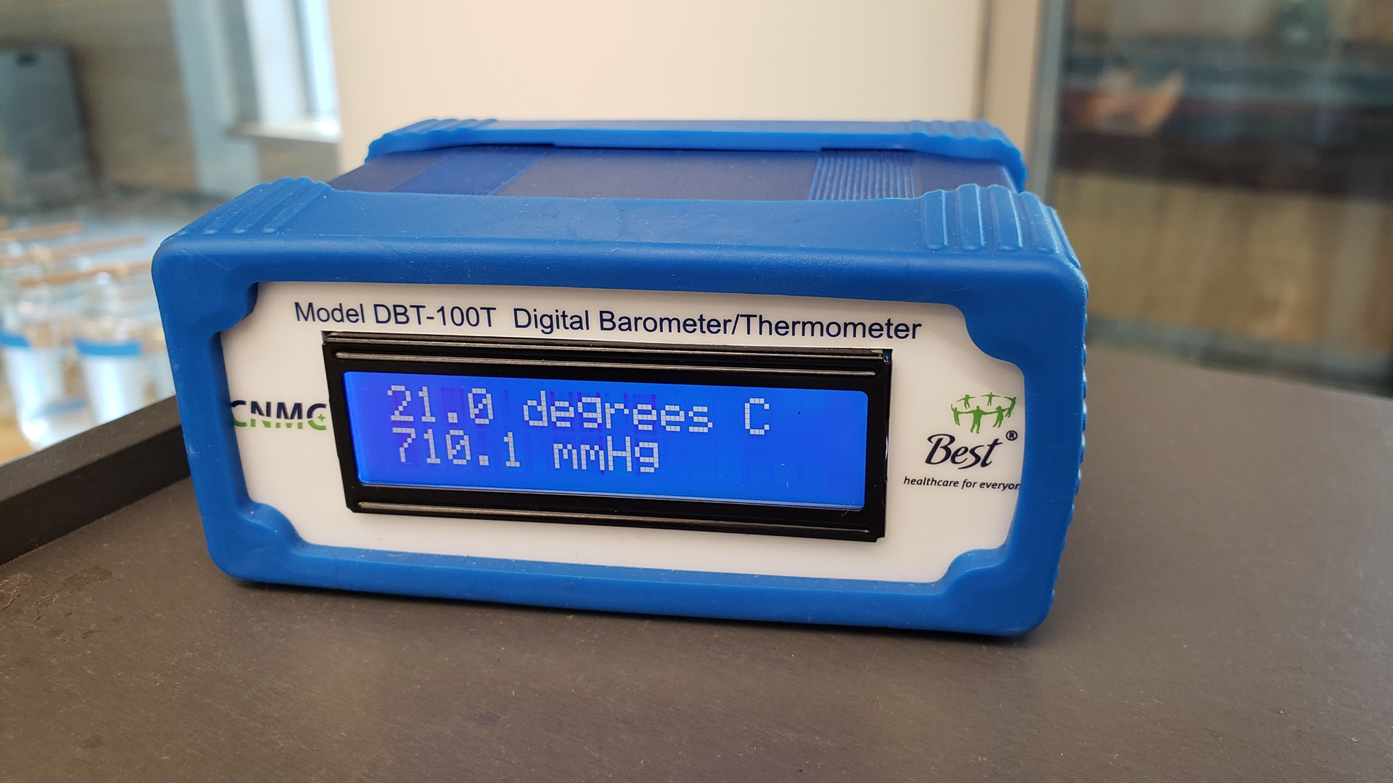
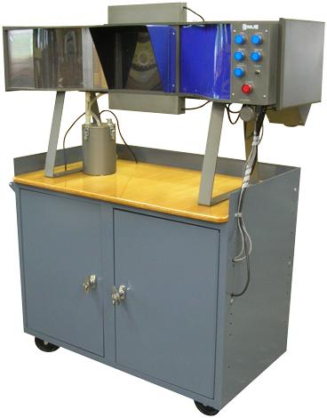
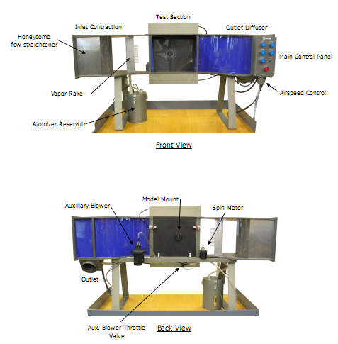
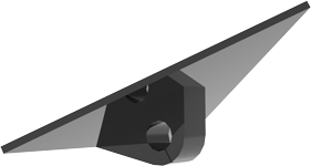
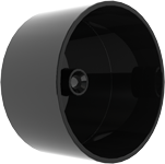
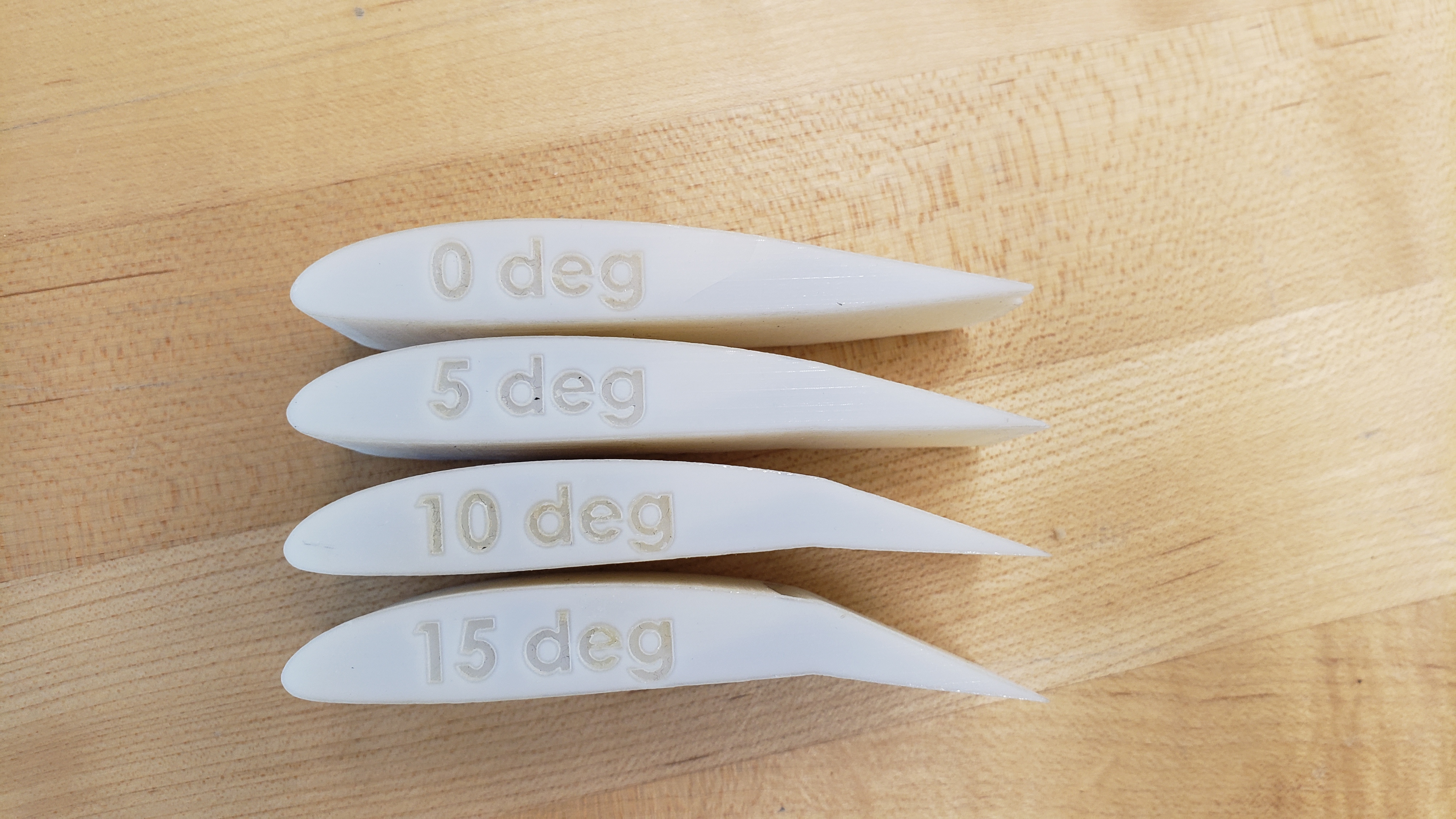
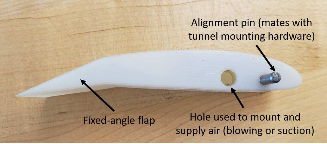
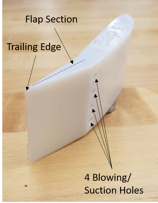
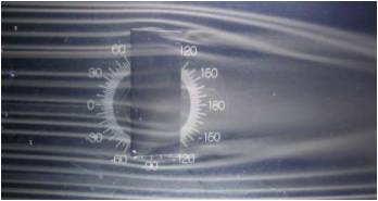
Figure 12. Sample smoke flow visualization for the airfoil model.

---